Standard Deviation Density Contribution Tool
Density Contribution Analysis
Density by Standard Deviation Intervals
Peak Density Zones
Density Statistics
Density Interpretation
The sd density contribution calculator is a specialized tool that examines the height of the normal distribution curve at critical points: the mean, ±1 SD, ±2 SD, and ±3 SD. It reveals how density—the curve’s height—decreases from the center, shaping the bell’s iconic form.
This focuses purely on density, the instantaneous height at a point, not area-based probability or variance. Density shows the relative likelihood concentration, highest at the mean and dropping outward. It’s vital for grasping why most data clusters centrally, clarifying bell curve density drop-off.
Unlike probability (area) or variance (spread), this tool spotlights curve height interpretation. For students, it demystifies Gaussian density function basics. To explore how variance and SD zones contribute to spread, see our Standard Deviation Percentage Contribution Calculator and Variance Distribution Analyzer.
What Is Density in a Normal Distribution?
Density in a normal distribution represents the height of the curve at any point, indicating concentration of likelihood. For a standard normal (mean=0, SD=1), the density formula is f(x) = (1 / √(2π)) * e^(-x²/2), peaking at ~0.3989 at the mean.
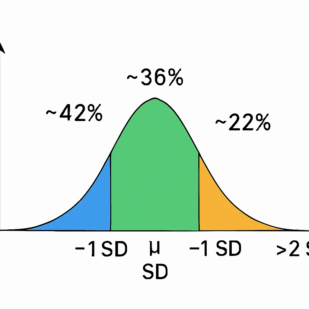
As you move to ±1 SD, density drops to ~0.242, about 60% of peak. At ±2 SD, it’s ~0.054, and by ±3 SD, ~0.004—nearly flat. This density behavior across SD shows rapid fall-off, creating the bell’s taper.
Density isn’t probability—probability is area under the curve, like the empirical rule’s 68% within ±1 SD. Density is height, not shaded region.
How the SD Density Contribution Tool Works
The sd density contribution calculator computes curve heights at specific SD points, showing their role in the distribution’s shape.
It works by:
Using mean and SD inputs (defaults to standard normal if omitted).
Calculating density at the mean (0 SD), ±1 SD, ±2 SD, and ±3 SD via the Gaussian formula.
Comparing each to peak density, expressing as percentages (e.g., ±1 SD at ~61% of max).
Interpreting contributions: High central density shapes the peak; low outer density flattens tails.
Outputting values with explanations, like “Density at ±2 SD is low, contributing to gentle slopes.”
It clarifies height of normal distribution, not areas or spreads—focusing on normal curve peak density and drop.
Density Values at Key SD Points (Standard Normal Example)
For a standard normal distribution, density values are:
| SD Position | Density Value f(x) | Contribution Interpretation |
|---|---|---|
| 0 SD | 0.3989 | Peak density, full height |
| ±1 SD | 0.24197 | ~61% of peak, noticeable drop |
| ±2 SD | 0.05399 | ~14% of peak, low height |
| ±3 SD | 0.00443 | ~1% of peak, almost flat |
These show density at mean and SD points, with exponential decline. Central height dominates shape; outer points barely register, explaining tail flatness.
This highlights standard normal density values, where curve steepness and spread stem from density fall-off.
Density Contribution vs Probability vs Variance (Key Differences)
Density, probability, and variance are related but distinct in normal distributions.
Density (this tool): Curve height at a point, like f(x), showing shape concentration. Highest at mean, drops outward.
Probability: Area under curve, like 68% within ±1 SD—measures likelihood ranges.
Variance: Squared deviations, emphasizing spread; outer points contribute more due to squaring.
Density sets the curve’s form, probability integrates it for chances, variance weights for variability.
(Even though density at 3 SD is extremely small, probability and variance behave differently — the area might be small, but the squared distance is large.)
Real-World Examples of Density Changes
In height distribution (μ=170 cm, σ=7 cm), density peaks at 170 cm, where most heights cluster—high curve height reflects common averages. At ±1 SD (163–177 cm), density drops, showing fewer extremes.
For test scores (μ=75, σ=10), the curve’s peak at 75 indicates average performance density; at ±2 SD (55 and 95), low height means rare high/low scores, flattening the bell.
In manufacturing precision, density at the target mean is high for accurate parts; at ±3 SD, near-zero height signals rare defects, explaining quality control focus on central consistency.
These illustrate density contribution by region, with central peak driving the bell’s form.
Why This Tool Is Important
This tool demystifies normal distribution height formula, teaching why the curve peaks sharply and tapers.
It clarifies density vs probability misconceptions, aiding deeper statistics grasp. For educators, it visualizes curve height interpretation; analysts see why outliers don’t spike density but affect tails.
Complements SD band variance behavior tools, enhancing data literacy.
FAQs
Related Tools
For variance insights, explore our Standard Deviation Percentage Contribution Calculator. Analyze distributions with the Variance Distribution Analyzer. See SD rankings in the Standard Deviation Importance Score Calculator. Learn contributions from Understanding Percentage Contribution of Standard Deviations in a Distribution. Start with basics at our Empirical Rule Calculator.
Conclusion
The sd density contribution calculator uncovers normal curve heights at key SD points, showing density’s rapid drop from peak to tails. This emphasizes central concentration, clarifying density vs probability distinctions.
Density shapes the bell, offering unique insights into distribution form. Experiment with density values for clearer understanding.
Empirical Rule Zones Probability Tool
Estimate probabilities within 1, 2, or 3 standard deviations using the 68-95-99.7 rule, with shaded bell curve visuals.
Try CalculatorEmpirical Rule Confidence Interval Calculator
Estimate data ranges using the 68-95-99.7 rule. Enter mean and SD to get ±1σ, ±2σ, or ±3σ intervals instantly.
Try CalculatorConfidence Interval from Mean and Standard Deviation Calculator
Compute exact confidence intervals from sample data. Input mean, SD, and sample size for 90%, 95%, or 99% CI.
Try CalculatorMargin of Error Using Empirical Rule Calculator
Find margin of error with the Empirical Rule. Enter mean and SD to get ±1σ, ±2σ, or ±3σ error bounds.
Try Calculator