Empirical Rule Calculator - 68 95 99.7 Rule of Normal Distribution
Input Parameters
Results
Normal Distribution Visualization
About the Empirical Rule
Within 1σ
About 68% of values lie within one standard deviation of the mean
Within 2σ
About 95% of values lie within two standard deviations of the mean
Within 3σ
About 99.7% of values lie within three standard deviations of the mean
Use this free calculator to find what percentage of your data falls within one, two, or three standard deviations of the mean. Just enter your dataset’s average and standard deviation to see how your values are distributed. This tool is perfect for students, data analysts, researchers, and anyone working with normally distributed data.
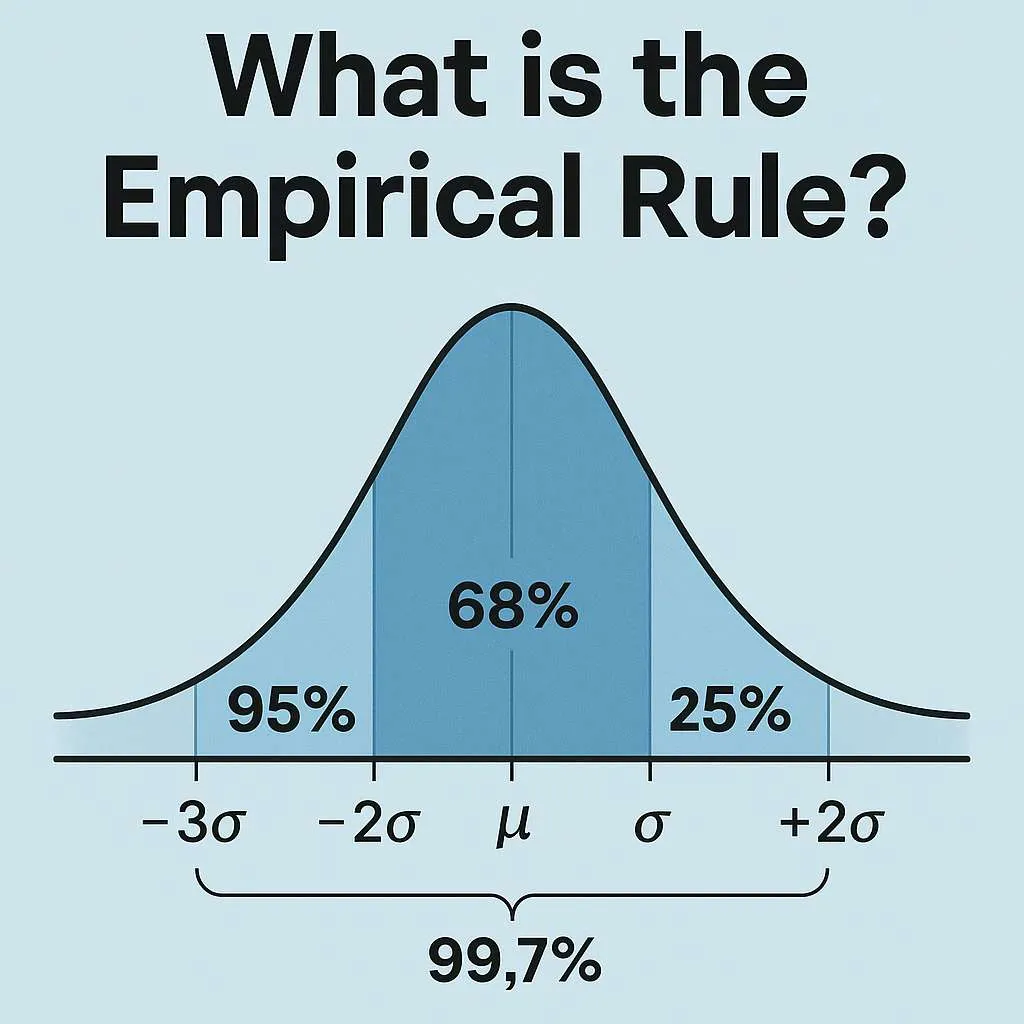
What is the Empirical Rule?
The empirical rule is a statistical shortcut that tells you how data spreads out in a bell-shaped pattern. If your data follows a normal distribution, you can predict where most values will fall without doing complex math.
Here’s what the rule tells us:
- 68% of values fall within one standard deviation of the average
- 95% fall within two standard deviations
- 99.7% fall within three standard deviations
This pattern shows up everywhere in nature and society—from people’s heights to test scores to manufacturing measurements. The rule gets its name from being based on empirical (observed) data rather than pure theory.
Why It Matters
Understanding this pattern helps you:
- Quickly estimate probabilities
- Spot unusual values in your data
- Make predictions about future measurements
- Determine if your data is normally distributed
- Set quality control standards
The rule only works when your data creates a symmetrical bell curve. If your data is heavily skewed to one side or has multiple peaks, you’ll need different statistical methods.
The Formula Explained
The math behind this rule is straightforward. You’re simply adding and subtracting standard deviations from your mean.
Basic Structure:
68% range: μ ± 1σ
95% range: μ ± 2σ
99.7% range: μ ± 3σ
Where:
- μ (mu) = your dataset’s mean or average
- σ (sigma) = standard deviation (how spread out your data is)
Breaking It Down:
| Coverage | Lower Limit | Upper Limit | Percentage |
|---|---|---|---|
| 1 Standard Deviation | μ − σ | μ + σ | 68% |
| 2 Standard Deviations | μ − 2σ | μ + 2σ | 95% |
| 3 Standard Deviations | μ − 3σ | μ + 3σ | 99.7% |
To find your specific ranges, take your mean and add/subtract the standard deviation multiplied by 1, 2, or 3.
How to Use This Tool (Step-by-Step Guide)
Follow these simple steps to analyze your data:
Step 1: Gather Your Numbers
You need two pieces of information:
- Your dataset’s mean (average of all values)
- The standard deviation (measure of spread)
Most statistical software and spreadsheets can calculate these automatically.
Step 2: Calculate Your Ranges
Plug your numbers into the formulas:
- 68% range: Mean – 1(SD) to Mean + 1(SD)
- 95% range: Mean – 2(SD) to Mean + 2(SD)
- 99.7% range: Mean – 3(SD) to Mean + 3(SD)
Step 3: Interpret What You Find
These ranges show you where to expect most of your data. Values outside the 95% range are unusual, and anything beyond 99.7% is extremely rare.
Complete Example: Test Scores
Imagine analyzing exam results where:
- Mean score = 75
- Standard deviation = 10
Let’s calculate each range:
One standard deviation (68%):
- Lower: 75 – 10 = 65
- Upper: 75 + 10 = 85
- Meaning: About 68% of students scored between 65 and 85
Two standard deviations (95%):
- Lower: 75 – 20 = 55
- Upper: 75 + 20 = 95
- Meaning: About 95% of students scored between 55 and 95
Three standard deviations (99.7%):
- Lower: 75 – 30 = 45
- Upper: 75 + 30 = 105
- Meaning: Nearly all students (99.7%) scored between 45 and 105
Any student scoring below 55 or above 95 performed unusually compared to their classmates.
Using Z-Scores
Want to know where a specific value falls? Calculate its Z-score:
Z = (Value – Mean) / Standard Deviation
For a score of 90: Z = (90 – 75) / 10 = 1.5
This student scored 1.5 standard deviations above average, placing them in roughly the top 7% of the class.
Real-World Applications
This statistical concept appears in countless practical situations. Here are some common examples:
Example 1: Intelligence Testing
IQ tests are designed around a normal distribution:
- Mean = 100
- Standard deviation = 15
What this means:
- 68% of people score between 85 and 115
- 95% score between 70 and 130
- 99.7% score between 55 and 145
Someone with an IQ of 130 (two standard deviations above average) is in the top 2.5% of the population. This is often the threshold for “gifted” programs.
Example 2: Human Height
Adult women’s heights in the US follow this pattern:
- Mean = 64 inches (5’4″)
- Standard deviation = 2.5 inches
Height distribution:
- 68% of women are between 61.5″ and 66.5″ (5’1.5″ to 5’6.5″)
- 95% are between 59″ and 69″ (4’11” to 5’9″)
- 99.7% are between 56.5″ and 71.5″ (4’8.5″ to 5’11.5″)
Women taller than 5’9″ represent only about 2.5% of the population, which explains why “tall” clothing sizes are specialty items.
Example 3: Quality Control in Manufacturing
A beverage company fills bottles targeting:
- Target volume = 500 ml
- Standard deviation = 5 ml
Production analysis:
- 68% of bottles contain between 495 and 505 ml
- 95% contain between 490 and 510 ml
- 99.7% contain between 485 and 515 ml
If regulations require bottles to contain at least 495 ml, the company knows approximately 16% of production falls below this threshold (the lower half of the 68% range). They can adjust their process to reduce variation and meet standards.
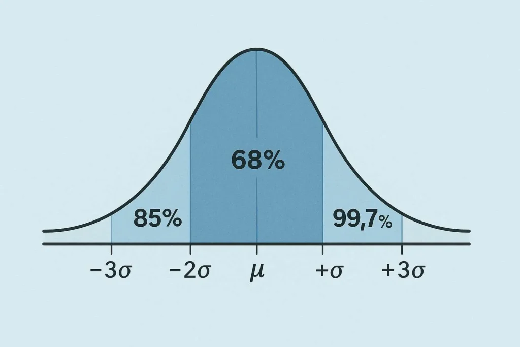
Understanding the Bell Curve Visualization
The normal distribution creates a distinctive bell-shaped curve that makes the empirical rule easy to visualize.
The Shape
Picture a symmetrical hill:
- The peak sits at the mean—this is where most data points cluster
- The slopes taper off gradually on both sides
- The tails extend infinitely in both directions but contain very few values
The Shaded Regions
When you use the tool above, you’ll see the curve divided into sections:
Central region (darkest shade): This middle section spanning one standard deviation on each side of the mean contains 68% of all data. It represents typical, everyday values.
Middle region (medium shade): Extending to two standard deviations captures an additional 27% of data (totaling 95%). These values are less common but still normal.
Outer region (lightest shade): The area between two and three standard deviations adds another 4.7% (bringing the total to 99.7%). Values here are unusual but not impossible.
The tails: The tiny slivers beyond three standard deviations contain only 0.3% of data—these are your extreme outliers.
Reading Your Results
The visual helps you instantly see:
- Whether a value is typical (inside the first band)
- If something is unusual enough to investigate (beyond two standard deviations)
- When a measurement is so extreme it might indicate an error (beyond three standard deviations)
Frequently Asked Questions
It means that in a bell-shaped data distribution, about 68% of values fall close to the average (within one standard deviation), 95% fall moderately close (within two standard deviations), and virtually all values (99.7%) fall within three standard deviations. Think of it as a way to describe how “bunched up” or “spread out” your data is.
Use it when your data is roughly bell-shaped and symmetrical. This applies to many natural measurements like heights, weights, test scores, and measurement errors. Before applying the rule, create a histogram of your data. If it looks approximately bell-shaped without severe skewing or multiple peaks, you’re good to go.
Both describe data spread, but they work differently. The empirical rule gives you precise percentages (68%, 95%, 99.7%) but only works for normal distributions. Chebyshev’s theorem works for any distribution but gives looser guarantees—it says at least 75% of data falls within two standard deviations (versus 95% for the empirical rule). Use the empirical rule when you have bell-shaped data; use Chebyshev’s when you’re unsure about the distribution.
They’re very close approximations. The precise values are 68.27%, 95.45%, and 99.73%, which we round for convenience. For perfectly normal distributions, these percentages are accurate. For real-world data that’s approximately normal, they’re excellent estimates.
Standard deviation measures how spread out your data is. A small standard deviation means most values cluster tightly around the average. A large standard deviation means values are scattered more widely. If test scores have a mean of 75 and a standard deviation of 3, most scores are very close to 75. If the standard deviation is 15, scores vary much more dramatically.
No—it’s specifically designed for normally distributed (bell-shaped) data. If your data is skewed, has multiple peaks, or follows a different pattern, the percentages won’t be accurate. Always check your data’s shape before applying the rule. Other distributions require different statistical methods.
Related Resources
- What Is the Empirical Rule: A detailed explanation of the 68-95-99.7 rule.
- How to Use the Empirical Rule on a Calculator: Step-by-step guide to mastering this tool.
- Empirical Rule vs. Chebyshev’s Theorem: Compare these statistical tools for better analysis.
- Applications of the Empirical Rule in Statistics and Probability: Discover real-world uses.
- Normal Distribution and the Empirical Rule: Comprehensive insights into normal distributions.
- All Tools: Browse our full collection of statistical calculators.
Check Our Other Tools:
Empirical Rule Graph Generator
Visualize the 68-95-99.7 Rule with a bell curve showing standard deviation intervals. Great for quick insights and presentations.
Try CalculatorBell Curve Generator
Create customizable bell curve plots for any normal distribution. Perfect for data analysis and visual reports.
Standard Deviation Shading Calculator
Shade areas under the curve based on standard deviation. Instantly see data coverage between values.
Try CalculatorZ-Score to Graph Plotter
Plot Z-scores on a bell curve and see where your value lies. Understand percentiles and probabilities at a glance.
Try CalculatorEmpirical Rule Percentile Calculator
Quickly estimate percentiles in a normal distribution using the 68-95-99.7 rule. Input mean, standard deviation, and a score to find its percentile rank.
Try CalculatorZ-Score to Percentile Converter
Convert a z-score to a percentile in a normal distribution. Enter your z-score to see the percentage of data below it, ideal for test scores or analytics.
Try CalculatorPercentile Rank Calculator
Find your score’s percentile rank without needing mean or standard deviation. Input your score and rank to see where you stand in any dataset.
Try CalculatorNormal Distribution to Percentile Visualizer
Visualize your score on a bell curve with shaded percentile areas. Enter mean, standard deviation, and a score to see its rank in a normal distribution.
Try CalculatorEmpirical Rule Probability Finder
Calculate probabilities under a normal distribution using the 68-95-99.7 rule with easy inputs and visual bell curve outputs.
Try CalculatorLeft/Right Tail Probability Calculator
Find left or right tail probabilities in a normal distribution using z-scores, perfect for hypothesis testing and p-values.
Try CalculatorProbability to Z-Score Approximation Tool
Convert cumulative probabilities to z-scores in a normal distribution, ideal for test scores and data analysis.
Try CalculatorEmpirical Rule Zones Probability Tool
Estimate probabilities within 1, 2, or 3 standard deviations using the 68-95-99.7 rule, with shaded bell curve visuals.
Try CalculatorEmpirical Rule Confidence Interval Calculator
Estimate data ranges using the 68-95-99.7 rule. Enter mean and SD to get ±1σ, ±2σ, or ±3σ intervals instantly.
Try CalculatorConfidence Interval from Mean and Standard Deviation Calculator
Compute exact confidence intervals from sample data. Input mean, SD, and sample size for 90%, 95%, or 99% CI.
Try CalculatorMargin of Error Using Empirical Rule Calculator
Find margin of error with the Empirical Rule. Enter mean and SD to get ±1σ, ±2σ, or ±3σ error bounds.
Try CalculatorEmpirical Rule Confidence Zone Visualizer
Empirical Rule Confidence Zone Visualizer Visualize 68-95-99.7 zones on a bell curve. Enter mean and SD to see shaded 1σ, 2σ, and 3σ areas.
Try CalculatorEmpirical Rule Range Probability Calculator
Estimate range probability between two values using the Empirical Rule (68-95-99.7). Ideal for quick normal distribution approximations without z-scores.
Try CalculatorEmpirical Rule Middle % Probability Calculator
Calculate middle percentages like 68% or custom central ranges in normal distributions with the Empirical Rule. Perfect for visualizing data clustering around the mean.
Try CalculatorEmpirical Rule Symmetric Interval Calculator
Find probabilities for symmetric intervals like mean ± k with the Empirical Rule. Explore central ranges in normal distributions for balanced probability estimates.
Try CalculatorEmpirical Rule Custom Zone Calculator
Empirical Rule Custom Zone Calculator Create and calculate custom zones like -3σ to -1σ in normal distributions using the Empirical Rule. Approximate probabilities for segmented bell curve analysis.
Try CalculatorEmpirical Rule Outlier Detector
Quickly identify mild and extreme outliers using ±2σ and ±3σ thresholds in normal distributions, with Z-scores and bell curve visuals for clear analysis.
Try CalculatorOutlier Threshold Calculator (Mean ± k·SD Tool)
Customize outlier boundaries with any k-value for flexible detection, ideal for analysts adjusting sensitivity in datasets like exam scores or quality checks.
Try CalculatorNormality Check Before Outlier Detection Tool
Assess if your data fits a normal distribution via skewness, kurtosis, and histograms—essential before applying empirical rule methods to avoid errors.
Try CalculatorEmpirical Rule Extreme Value Finder
Rank data points by extremeness beyond 2 SD, 2.5 SD, and 3 SD, classifying them as moderately extreme, very extreme, or highly unusual with tail visualizations.
Try CalculatorStandard Deviation Percentage Contribution Calculator
Break down variance in normal distributions by SD bands (0–1σ, 1–2σ, etc.), revealing each zone's share of total spread with clear examples and insights.
Try CalculatorVariance Distribution Analyzer
Analyze how variance distributes across SD zones in normal curves, highlighting contributions from central, middle, and tail regions for deeper data understanding.
Try CalculatorSD Density Contribution Tool
Examine normal curve heights at key SD points (mean, ±1σ, ±2σ, ±3σ), explaining density drop-off and its role in shaping the bell curve.
Try CalculatorSD Importance Score Calculator
Rank SD zones by importance using density, variance, and spread factors, offering conceptual scores to prioritize analysis in distributions.
Try Calculator