Normal Distribution and the Empirical Rule: Complete Guide
The normal distribution, often visualized as a bell-shaped curve, is a cornerstone of statistics, describing how data like test scores or heights spreads around an average. The empirical rule, also known as the 68-95-99.7 rule, is a powerful tool for analyzing this distribution, revealing that 68%, 95%, and 99.7% of data fall within one, two, and three standard deviations of the mean, respectively. This guide dives deep into the normal distribution and empirical rule, offering insights, examples, and practical tips for students, educators, and analysts. Whether you’re new to statistics or brushing up, this guide will help you master these concepts and apply them effectively.
What Is a Normal Distribution?
A normal distribution is a symmetric, bell-shaped pattern where most data clusters near the mean (average), with fewer values at the extremes. It’s defined by two parameters:
Mean (μ): The center of the distribution, representing the average.
Standard Deviation (σ): A measure of how spread out the data is.
Normal distributions are common in real-world data, like IQ scores, weights, or delivery times, making them essential for statistical analysis. The bell curve’s symmetry means half the data lies below the mean and half above, creating a predictable pattern.
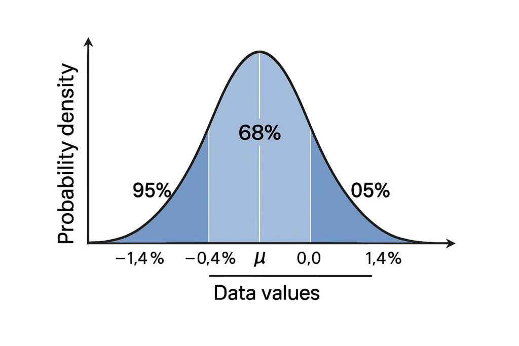
The Empirical Rule Explained
The empirical rule is a shortcut for understanding normal distributions. It states:
68% of data falls within one standard deviation (μ ± 1σ).
95% falls within two standard deviations (μ ± 2σ).
99.7% falls within three standard deviations (μ ± 3σ).
This rule helps estimate probabilities and percentages quickly without complex calculations. For example, in a dataset of heights, most values cluster near the mean, and the empirical rule quantifies how much data lies in each range.
For a foundational overview, check out what the empirical rule is.
The Empirical Rule Formula
The empirical rule is expressed through simple intervals:
μ ± 1σ → 68%: 68% of data lies within one standard deviation of the mean.
μ ± 2σ → 95%: 95% of data is within two standard deviations.
μ ± 3σ → 99.7%: 99.7% of data falls within three standard deviations.
These percentages are specific to normal distributions, making the rule a go-to for quick analysis.
| Range | Percentage | Example (μ = 100, σ = 10) |
|---|---|---|
| μ ± 1σ | 68% | 90 to 110 |
| μ ± 2σ | 95% | 80 to 120 |
| μ ± 3σ | 99.7% | 70 to 130 |
Real-World Applications of the Empirical Rule
The normal distribution empirical rule calculator simplifies data analysis in various fields. Here are three practical examples:
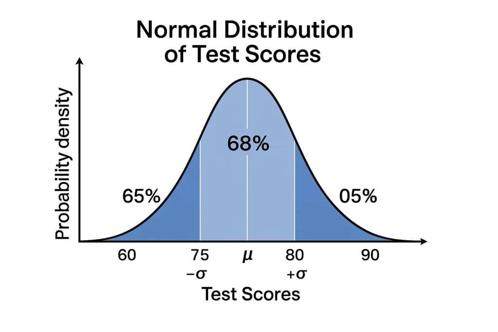
Example 1: Test Scores
A class’s exam scores have a mean of 80 and a standard deviation of 5. Using the empirical rule:
68% of students score between 75 and 85.
95% score between 70 and 90.
99.7% score between 65 and 95.
This helps teachers set grading curves or identify outliers. For instance, a score of 90 is in the top 2.5%, indicating exceptional performance.
Example 2: Heights of Adults
Adult female heights in a region have a mean of 65 inches and a standard deviation of 2.5 inches. The empirical rule shows:
68% of women are between 62.5 and 67.5 inches.
95% are between 60 and 70 inches.
99.7% are between 57.5 and 72.5 inches.
This is useful for industries like fashion or healthcare to design products or set health benchmarks.
Example 3: Delivery Times
A courier service’s delivery times have a mean of 30 minutes and a standard deviation of 4 minutes. Using an empirical rule bell curve calculator:
68% of deliveries take 26 to 34 minutes.
95% take 22 to 38 minutes.
99.7% take 18 to 42 minutes.
This helps businesses optimize logistics and manage customer expectations.
When to Use the Empirical Rule
The empirical rule is ideal when:
Data is approximately normal, forming a bell-shaped curve.
You have a large sample (30+ observations) to ensure normality.
You need quick estimates of probabilities or percentages.
It’s perfect for fields like education, biology, or finance where normal distributions are common. To apply it to your data, try our empirical rule calculator.
Limitations of the Empirical Rule
The empirical rule is powerful but has limits:
Normal Data Only: It doesn’t apply to skewed or bimodal distributions, like income or time-to-failure data.
Sample Size: Small datasets may not be normal, reducing accuracy.
Approximation: The 68-95-99.7% figures assume perfect normality, which real data may not fully meet.
Outliers: Extreme values can skew the mean or standard deviation, affecting results.
Use histograms or normality tests to confirm your data is bell-shaped before applying the rule.
Comparing the Empirical Rule to Other Tools
The empirical rule is specific to normal distributions, unlike Chebyshev’s Theorem, which applies to any dataset but offers less precise estimates (e.g., at least 75% within ±2σ vs. 95% for the empirical rule). The empirical rule’s precision makes it ideal for bell-shaped data, while Chebyshev’s is better for non-normal data.
Frequently Asked Questions (FAQs)
It’s a bell-shaped curve where data clusters symmetrically around the mean, common in datasets like heights or test scores.
It estimates that 68%, 95%, and 99.7% of data fall within one, two, and three standard deviations of the mean, respectively.
Yes, it computes percentages or probabilities for normal data based on the mean and standard deviation.
It doesn’t work for skewed, non-normal, or small datasets (fewer than 30 observations).
It represents normal distributions, which are common in real-world data, making the empirical rule a key analysis tool.
Conclusion
The normal distribution and empirical rule are essential for understanding data patterns in statistics. The 68-95-99.7 rule simplifies analyzing bell-shaped datasets, from test scores to delivery times, offering quick insights into probabilities and percentages. While limited to normal distributions, it’s a powerful tool for students, researchers, and analysts. Use our empirical rule calculator to explore your data, and dive into what the empirical rule is for foundational knowledge. With this guide, you’re equipped to master normal distributions and apply the empirical rule confidently.
Other Resources:
- What Is the Empirical Rule: A detailed explanation of the 68‑95‑99.7 rule.
- How to Use the Empirical Rule on a Calculator: Step-by-step guide to mastering this tool.
- Empirical Rule vs. Chebyshev’s Theorem: Compare these statistical tools for better analysis.
- Applications of the Empirical Rule in Statistics and Probability: Discover real-world uses.
- All Tools: Browse our full collection of statistical calculators.