How to Identify Outliers Using the Empirical Rule (68–95–99.7%)
Outliers are data points that differ significantly from other observations in a dataset. They might represent errors, variability, or important anomalies. The empirical rule, also known as the 68-95-99.7 rule, offers a quick way to identify outliers empirical rule style by checking how far a value is from the mean in terms of standard deviations. This method is especially useful for normal distributions, where data forms a symmetric bell curve.
It’s a beginner-friendly approach for spotting potential issues in datasets like test scores or heights. However, remember that empirical rule outlier identification only works well for data that’s approximately normal. For hands-on practice, check out our Empirical Rule Calculator or the Empirical Rule Outlier Detector to automate the process.
What Counts as an Outlier Using the Empirical Rule?
The empirical rule helps define outliers based on where data falls in a normal distribution. In such distributions:
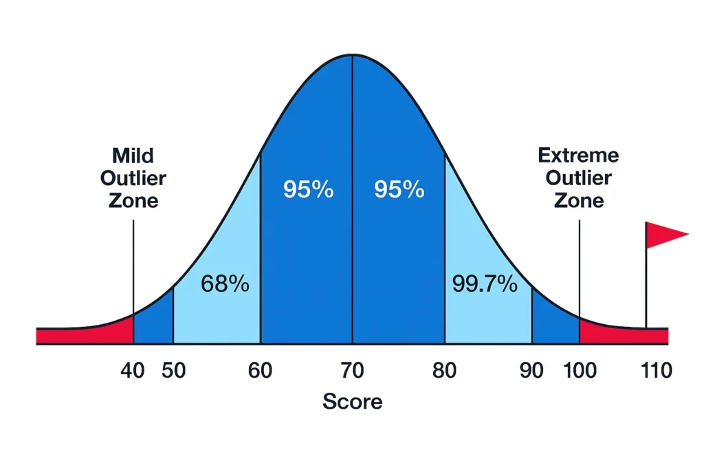
- About 68% of values are within ±1 standard deviation (σ) of the mean.
- Roughly 95% are within ±2σ.
- Approximately 99.7% are within ±3σ.
This means most data clusters close to the mean, with fewer points farther out. For outlier detection:
- Mild Outlier: Values between ±2σ and ±3σ. These are unusual but not rare enough to be extreme. They fall in the outer 4.7% of the data (beyond the central 95% but within 99.7%).
- Extreme Outlier: Values beyond ±3σ. These are very rare, occurring in only about 0.3% of the data, making them outliers beyond 3 standard deviations.
This classification provides a standard deviation outlier threshold for quick checks. For automated classification, try the Empirical Rule Outlier Detector
Step-by-Step: How to Identify Outliers With the Empirical Rule
Identifying outliers using the empirical rule is straightforward. Follow these steps with a real-world example to see empirical rule 68 95 99.7 outliers in action.
Step 1: Calculate the Mean (μ)
The mean is the average of your dataset. Add all values and divide by the number of observations.
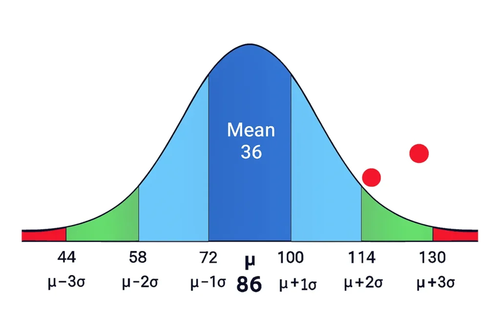
Example Dataset (test scores for a class of 10 students): 70, 75, 78, 80, 82, 85, 88, 90, 92, 120. Mean (μ) = (70 + 75 + 78 + 80 + 82 + 85 + 88 + 90 + 92 + 120) / 10 = 86.
Step 2: Calculate the Standard Deviation (σ)
Standard deviation measures data spread. Use the formula: σ = sqrt[Σ(x – μ)² / n] for a population, or divide by (n-1) for a sample.
For our example (using sample SD): σ ≈ 14.5 (calculated via spreadsheet or calculator).
Step 3: Convert the Suspicious Value to a Z-Score
The Z-score shows how many standard deviations a value (X) is from the mean: Z = (X – μ) / σ.
For the suspicious value 120: Z = (120 – 86) / 14.5 ≈ 2.34.
Step 4: Interpret Using Empirical Thresholds
Compare the Z-score to the rule:
- |Z| < 2: Not an outlier (within 95% of data).
- 2 ≤ |Z| < 3: Mild outlier.
- |Z| ≥ 3: Extreme outlier.
In our example, Z ≈ 2.34 indicates a mild outlier. It’s unusual but not extreme. For a value like 130: Z = (130 – 86) / 14.5 ≈ 3.03 → extreme outlier.
This z-score outlier check makes empirical rule outlier identification precise and easy.

Why the Empirical Rule Works for Outlier Detection
The empirical rule leverages the properties of normal distributions, where data is symmetric around the mean. In a bell curve, values naturally taper off, so outliers fall in the extreme tails—beyond where 99.7% of data lies.
This makes it effective for normal distribution outlier detection because rare events (less than 0.3% chance) often signal anomalies. It’s a fast, approximate outlier detection method for early screening in fields like quality control or research, without needing advanced software.
For instance, in height measurements (mean 68 inches, SD 3 inches), a height of 80 inches (Z ≈ 4) would be an extreme outlier, possibly indicating a measurement error.
Empirical Rule vs IQR Method (Comparison)
The empirical rule is one way to spot outliers, but it’s not always the best. Here’s a comparison with the Interquartile Range (IQR) method, which is more robust.
| Feature | Empirical Rule | IQR Method |
|---|---|---|
| Uses SD & mean | Yes | No |
| Requires normality | Yes | No |
| Works for skewed data | No | Yes |
| Best for | Normal distributions | Any distribution |
| Outlier threshold | ±2σ (mild), ±3σ (extreme) | Q1 − 1.5×IQR & Q3 + 1.5×IQR |
The empirical rule shines for bell curve outlier examples but can fail on skewed data. This is why it’s important to check normality using the Normality Check Before Outlier Detection Tool.
The IQR method, based on quartiles, handles mild vs extreme outliers in non-normal data better, making it a good alternative.
When NOT to Use the Empirical Rule to Identify Outliers
While handy, the empirical rule has limitations and shouldn’t be used in certain cases:
- Highly Skewed Distributions: Data like incomes (pulled by high earners) won’t follow the 68-95-99.7 pattern, leading to false flags.
- Bimodal or Multimodal Data: Datasets with two or more peaks (e.g., combined male/female heights) distort the bell curve.
- Heavy-Tailed Distributions: Data with frequent extremes (e.g., stock returns) makes ±3σ thresholds unreliable.
- Very Small Sample Sizes: With fewer than 30 observations, normality isn’t assured, causing empirical rule limitations.
- Data with Extreme Variance: If variance is inconsistent, the rule over- or underestimates outliers.
In these scenarios, you risk misidentifying normal values as outliers or missing real ones. For non-normal data, consider IQR or robust statistical methods instead. Always verify the normality assumption for outliers first.
Visual Bell Curve Example
A visual helps grasp how outliers appear on a bell curve. Imagine a normal distribution of IQ scores: mean (μ) = 100, standard deviation (σ) = 15.
- The curve peaks at 100.
- ±1σ: 85 to 115 (68% shaded green).
- ±2σ: 70 to 130 (95% shaded blue).
- ±3σ: 55 to 145 (99.7% shaded light blue).
Now, plot a red dot at 160 (Z = (160 – 100) / 15 ≈ 4), far in the right tail beyond +3σ. This is an extreme outlier—extremely rare in a normal IQ distribution.
FAQs
Typically, 2 or more standard deviations indicate a mild outlier, while 3 or more signal an extreme one under the empirical rule.
In normal distributions, yes—values beyond ±3σ are extreme outliers, occurring in only 0.3% of data. But confirm normality first.
No, it’s unreliable for skewed data as the 68-95-99.7 percentages assume symmetry. Use IQR instead.
Mild outliers are between ±2σ and ±3σ (unusual, about 4.7% of data), while extreme ones are beyond ±3σ (rare, 0.3%).
Tools like our Empirical Rule Outlier Detector or Outlier Threshold Calculator automate the process with Z-scores and visuals.
Related Tools
Conclusion
The empirical rule provides a fast way to identify outliers empirical rule method in normal distributions, classifying values beyond ±2σ as mild outliers and beyond ±3σ as extreme. Through steps like calculating Z-scores, you can spot anomalies in datasets like test scores or heights efficiently. However, it’s an approximate method that relies on the normality assumption for outliers—always check this to avoid errors.
As a first-pass screening tool, it’s ideal for beginners, but pair it with methods like IQR for skewed data. Start identifying outliers instantly using the Empirical Rule Outlier Detector.
Empirical Rule Zones Probability Tool
Estimate probabilities within 1, 2, or 3 standard deviations using the 68-95-99.7 rule, with shaded bell curve visuals.
Try CalculatorEmpirical Rule Confidence Interval Calculator
Estimate data ranges using the 68-95-99.7 rule. Enter mean and SD to get ±1σ, ±2σ, or ±3σ intervals instantly.
Try CalculatorConfidence Interval from Mean and Standard Deviation Calculator
Compute exact confidence intervals from sample data. Input mean, SD, and sample size for 90%, 95%, or 99% CI.
Try CalculatorMargin of Error Using Empirical Rule Calculator
Find margin of error with the Empirical Rule. Enter mean and SD to get ±1σ, ±2σ, or ±3σ error bounds.
Try Calculator