Variance Distribution Analyzer
Variance Distribution Analysis
Variance by Standard Deviation Zones
Variance Concentration Analysis
Distribution Insights
The variance distribution calculator is a conceptual tool that analyzes how total variance spreads across key zones in a normal distribution, such as within ±1 SD, between 1–2 SD, and beyond 2 SD. It shows the percentage each zone contributes to variance—the average squared deviation from the mean—highlighting the “architecture” of spread.
This differs from probability tools, focusing instead on how squared distances amplify outer zones’ impact. For students, it clarifies why variance rises with extremes; for analysts, it aids data interpretation. Understanding variance distribution helps grasp distribution shape and variability’s true sources.
For a more detailed look at how SD zones contribute to variance, see our Standard Deviation Percentage Contribution Calculator.
What Is Variance Distribution?
Variance distribution refers to how a normal distribution’s total variance—the measure of data spread as average squared deviation from the mean—divides across SD zones. Each zone, like within ±1 SD or beyond 2 SD, contributes a unique share based on point density and deviation size.
Variance is the heart of statistical spread, quantifying variability. In a bell curve, central zones have high density but small deviations, yet their volume drives major variance. Outer zones, with low density but large squared deviations, add meaningfully despite rarity.
This isn’t probability—where the center holds 68% within 1 SD—but variance contribution, balancing frequency and distance. It reveals SD zone variance in action.
How the Variance Distribution Analyzer Works
The variance distribution analyzer simplifies exploring variance by SD zones in a normal distribution. Assuming symmetry and bell shape, it partitions the curve conceptually.
Assumes a Normal Distribution: Starts with mean (μ) and SD (σ) for theoretical breakdown.
Divides into SD Bands: Splits into within ±1 SD (central), 1–2 SD (middle), and beyond 2 SD (outer/tails).
Calculates Squared Deviation per Band: Weights deviations by density to find each zone’s variance share.
Converts to Percentages: Normalizes so sums equal 100%, with total variance as baseline (σ²=1 for standard normal).
Outputs Proportions: Shows easy-to-read % per zone, like ~42% central, ~58% outer combined.
It’s not a probability tool—empirical rule covers that—nor empirical rule percentages. It zeros in on variance by standard deviation, the core of understanding spread of data.
Why Variance Distribution ≠ Probability Distribution
Variance and probability both describe normal distributions but diverge in focus. Probability tallies likelihood—how many points fall where—while variance distribution weighs by squared deviation, emphasizing impact on spread.
In probability, within ±1 SD holds ~68%, 1–2 SD adds ~27%, beyond 2 SD is ~5%. Variance boosts outer zones because squaring amplifies distance, so beyond 2 SD contributes more than its tiny probability.
Centers dominate probability due to density; variance balances this with distance, making middle and tails punchier. This variance vs probability difference is key—probability for counting, variance for measuring influence.
While the probability beyond 2 SD is tiny (about 5%), the variance contribution beyond 2 SD is noticeably larger because extreme values are squared, amplifying their impact.
Example of Variance Distribution Across SD Zones
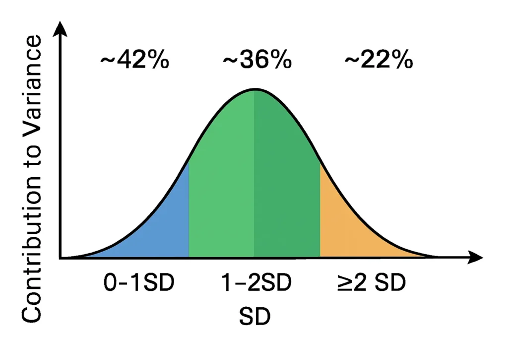
For a normal distribution, variance distribution approximates:
| SD Zone | Variance Contribution (Approx) |
|---|---|
| Within ±1 SD | ~42% |
| 1–2 SD | ~36% |
| Beyond 2 SD | ~22% |
The within ±1 SD leads with ~42%, as dense clustering yields high cumulative squared deviations. 1–2 SD follows at ~36%, blending moderate factors.
Beyond 2 SD contributes ~22%, showing tails’ role via extreme squares despite low probability. This normal distribution variance breakdown scales for any dataset.
In heights (μ=170 cm, σ=7 cm), within 163–177 cm drives most variance from common deviations.
Real-World Examples of Variance Distribution
In height distribution, within ±1 SD (e.g., 163–177 cm for μ=170, σ=7) contributes most variance—most people near average create steady spread through small but frequent deviations.
For test scores (μ=75, σ=10), 1–2 SD (65–85 and 85–95) adds significant variance, where moderate scores pull overall variability.
In measurement error for machine parts, beyond 2 SD shows rare large errors contributing noticeably to variance, explaining why outliers skew quality metrics.
These highlight SD band variance behavior, with central dominance and outer subtlety in everyday data.
Why This Tool Is Important
The variance distribution analyzer demystifies how variance is distributed, showing why extremes disproportionately affect SD despite rarity.
It aids teaching distribution density, helping educators illustrate squared deviation’s role. Analysts gain better data interpretation, seeing central vs outer influence.
This fosters understanding spread of data beyond basics, supporting empirical rule comparison for deeper insights.
FAQs
It’s how total variance divides across SD zones in a normal distribution, based on density and squared distance.
Central (within 1 SD) most, middle (1–2 SD) strongly, outer (beyond 2 SD) meaningfully but less.
Squaring extreme deviations amplifies their impact, outweighing rarity.
Empirical rule is probability-based; this is variance-weighted, emphasizing spread over frequency.
Squared deviation, focusing on variance structure, not point counts.
Related Tools
For precise breakdowns, use our Standard Deviation Percentage Contribution Calculator. Explore density with the Standard Deviation Density Contribution Tool. Analyze variances in the Variance Distribution Analyzer. Rank SD impacts via the Standard Deviation Importance Score Calculator. Start with basics at our Empirical Rule Calculator.
Conclusion
Z-Score to Percentile Converter
Convert a z-score to a percentile in a normal distribution. Enter your z-score to see the percentage of data below it, ideal for test scores or analytics.
Try CalculatorEmpirical Rule Probability Finder
Calculate probabilities under a normal distribution using the 68-95-99.7 rule with easy inputs and visual bell curve outputs.
Try CalculatorLeft/Right Tail Probability Calculator
Find left or right tail probabilities in a normal distribution using z-scores, perfect for hypothesis testing and p-values.
Try CalculatorProbability to Z-Score Approximation Tool
Convert cumulative probabilities to z-scores in a normal distribution, ideal for test scores and data analysis.
Try Calculator