Chebyshev’s theorem guarantees that at least (1 − 1/k²) × 100% of values in any distribution lie within k standard deviations of the mean, in [μ − kσ, μ + kσ]. At k = 2, at least 75% are inside; at k = 3, at least 88.89%. Use the Chebyshev’s theorem calculator above for any mean, standard deviation and k.
Unlike the empirical rule, which only works for bell-shaped normal data, Chebyshev’s theorem applies to every distribution — skewed, bimodal or completely unknown. It is also called Chebyshev’s inequality, or the Chebyshev bound, and it gives a minimum percentage rather than an exact one. Our empirical rule vs Chebyshev’s theorem guide explains the difference in full, while the bell curve generator shows what a normal curve looks like.
On this page you will find the free Chebyshev’s theorem calculator, the formula, a k table, a worked example for each mode and a comparison with the empirical rule — everything you need to use the Chebyshev bound in homework, exams and real data analysis. If you need the spread of your data first, our standard deviation calculator finds σ from any dataset.
What Is Chebyshev's Theorem?
Chebyshev’s theorem — also called Chebyshev’s inequality, or the Bienaymé–Chebyshev inequality — states that for any distribution with a finite mean μ and a finite standard deviation σ, the proportion of values within k standard deviations of the mean is at least 1 − 1/k² (for k > 1). In words: no matter how skewed or strangely shaped a dataset is, at least (1 − 1/k²) × 100% of its values fall inside the interval [μ − kσ, μ + kσ], and at most (1/k²) × 100% can fall outside it.
That makes Chebyshev’s theorem the safety net of statistics. When a dataset is bell-shaped, the empirical rule gives tighter, exact percentages (68.27% within 1σ, 95.45% within 2σ, 99.73% within 3σ); our guide to the empirical rule explains them. But when the shape is unknown, Chebyshev’s rule is the only statement you can safely make — see the full empirical rule vs Chebyshev’s theorem comparison on this page for the numbers side by side. The theorem is named after the Russian mathematician Pafnuty Chebyshev, and its foundation is documented in the NIST/SEMATECH e-Handbook of Statistical Methods.
Chebyshev's Theorem Formula
The Chebyshev’s theorem formula is:
P(|X − μ| ≥ kσ) ≤ 1/k² and P(|X − μ| < kσ) ≥ 1 − 1/k²
It says that the probability of a value falling k or more standard deviations from the mean is at most 1/k² — so the probability it lies inside [μ − kσ, μ + kσ] is at least 1 − 1/k². In the absolute form, with a distance d in the original units and variance σ², the Chebyshev bound is P(|X − μ| ≥ d) ≤ σ²/d² and P(|X − μ| < d) ≥ 1 − σ²/d².
- μ (mu) — the mean of the distribution.
- σ (sigma) — the standard deviation. Its square, σ², is the variance.
- k — how many standard deviations from the mean. k must be greater than 1 for a positive guarantee.
- d — a distance from the mean in the original units (absolute-bound mode).
If you need σ for your own data, see how to calculate standard deviation, and remember that a population and a sample use different denominators — our population vs sample standard deviation comparison explains which one to use before you plug σ into Chebyshev’s theorem.
How to Use the Chebyshev's Theorem Calculator
- Choose a mode. Use Standardized when you know the mean, the standard deviation and the number of sigmas (k). Use Absolute bound when you know the variance and a distance from the mean in the original units.
- Enter your values. In standardized mode, type the mean μ, the standard deviation σ and k (try k = 2 or k = 3). In absolute mode, type the mean μ, the variance σ² and the distance d. Add a sample size n if you want the minimum expected count inside the interval.
- Click Calculate. Read the minimum percentage inside, the maximum percentage outside, the interval and — if you entered n — the minimum expected count inside.
- Check the bound. Remember that Chebyshev’s bound is a minimum: the real percentage can be higher. For bell-shaped data, compare the result with the empirical rule confidence interval calculator to see how much tighter the 68–95–99.7 rule is when normality holds.
Worked Example: Standardized Mode (k in Standard Deviations)
Suppose the mean score on a test is μ = 60 with a standard deviation of σ = 8, and we want the range that holds at least 75% of the scores. Use k = 2:
1 − 1/k² = 1 − 1/2² = 1 − 0.25 = 0.75 → at least 75%
The interval is [μ − kσ, μ + kσ] = [60 − 2 × 8, 60 + 2 × 8] = [44, 76], and at most 25% of scores can fall outside it. With a sample of n = 100 students, at least 75 of them are expected inside [44, 76].
For k = 3 the guarantee is stronger: 1 − 1/3² = 1 − 1/9 = 0.8889, so at least 88.89% of values lie in [60 − 24, 60 + 24] = [36, 84]. The boundary μ ± kσ is the same idea as a z-score of ±k: here the interval [44, 76] is the set of values whose z-score is between −2 and +2.
Worked Example: Absolute Bound Mode (Variance and Distance)
Suppose a dataset has variance σ² = 3.75 and we want to know how many values can be 5 or more units from the mean. First, σ = √3.75 = 1.9365. Then:
P(|X − μ| ≥ 5) ≤ σ²/d² = 3.75/5² = 3.75/25 = 0.15 → at most 15%
So at least 85% of the values lie within 5 units of the mean — with a mean of 60, that is the interval [55, 65]. This is the same calculation the calculator does in the absolute-bound mode, and it works even when you only know the variance and not the shape of the distribution.
Chebyshev's Theorem k Table
The table below gives the minimum percentage inside and the maximum percentage outside for the most common k values. This is the same Chebyshev’s theorem k table the calculator works from, and these are the numbers worth remembering:
| k (standard deviations) | Minimum % inside | Maximum % outside |
|---|---|---|
| 1 | 0% | 100% |
| 1.5 | 55.56% | 44.44% |
| 2 | 75% | 25% |
| 2.5 | 84% | 16% |
| 3 | 88.89% | 11.11% |
| 4 | 93.75% | 6.25% |
| 5 | 96% | 4% |
Reading the table: at k = 2, at least 75% of values are within two standard deviations, and at most 25% can be outside. Notice that k = 1 gives a 0% guarantee — the bound only becomes useful once k is greater than 1. If you need the matching percentages for a bell-shaped curve instead, the empirical rule percentile calculator gives the 68.27%, 95.45% and 99.73% figures.
Chebyshev's Theorem vs the Empirical Rule
Chebyshev’s theorem and the empirical rule answer the same question — “how much data is within k standard deviations?” — but they make different assumptions. Chebyshev’s theorem works for any distribution; the empirical rule only works for normal data. The price of that guarantee is that Chebyshev’s percentages are minimums, so they are lower than the exact percentages a normal curve actually holds:
| Chebyshev’s theorem | Empirical rule | |
|---|---|---|
| Works for | Any distribution | Normal distributions only |
| k = 1 | ≥ 0% (no guarantee) | ≈ 68.27% |
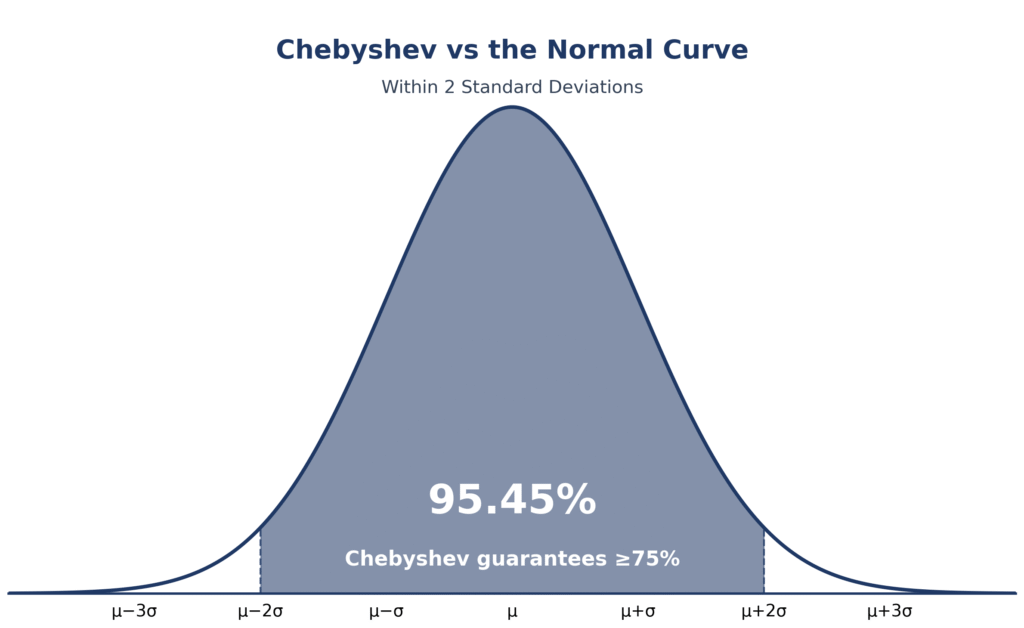
| k = 2 | ≥ 75% | ≈ 95.45% |
| k = 3 | ≥ 88.89% | ≈ 99.73% |
| Result type | Minimum (lower bound) | Actual percentage (approx.) |
For a normal distribution the empirical rule is tighter — 95.45% of values really are within 2σ, while Chebyshev only promises 75%. But if the distribution is skewed, the empirical rule can be badly wrong while Chebyshev’s bound stays true. To see the normal curve at k = 2, open the empirical rule graph generator; our normal distribution and empirical rule guide explains where the 68–95–99.7 figures come from.
Common Mistakes When Using Chebyshev's Theorem
- Using k ≤ 1 and expecting a guarantee. At k = 1 the bound is exactly 0%, and below 1 it is negative — Chebyshev’s theorem says nothing useful at or below one standard deviation. k must be greater than 1 for a positive guarantee.
- Treating the bound as the exact percentage. Chebyshev gives a minimum, not the actual share. At k = 2 the theorem guarantees at least 75% inside, but a normal dataset really has about 95.45% there. Confusing the minimum with the measured percentage is the most common error.
- Applying the empirical rule to non-normal data. If the distribution is not bell-shaped, the 68–95–99.7 percentages do not apply — only Chebyshev’s bound does.
- Mixing up variance and standard deviation. In the absolute form the input is the variance σ², not σ. With variance 3.75, the standard deviation is √3.75 = 1.9365 — not 3.75.
- Using a sample standard deviation where a population one is needed. Check which one your data uses (see the population vs sample standard deviation comparison) before plugging σ into the calculator.
What percentage is within 2 standard deviations according to Chebyshev's theorem?
According to Chebyshev’s theorem, at least 75% of the values in any distribution lie within 2 standard deviations of the mean, and at most 25% lie outside. The calculation is 1 − 1/2² = 1 − 0.25 = 0.75. This is a minimum: if the data is normally distributed, the actual share is about 95.45% (the empirical rule), but Chebyshev’s 75% is guaranteed no matter what shape the data has.
How do you use Chebyshev's theorem?
Find the mean μ and standard deviation σ of the data, choose a number of standard deviations k (greater than 1), then compute 1 − 1/k² — that is the minimum proportion of values inside [μ − kσ, μ + kσ]. For example, with μ = 60, σ = 8 and k = 2, at least 75% of values lie in [44, 76]. The Chebyshev’s theorem calculator above does the whole calculation and returns the interval and the maximum percentage outside.
What is the difference between Chebyshev's theorem and the empirical rule?
Chebyshev’s theorem guarantees a minimum percentage for any distribution — at least 75% within 2σ and 88.89% within 3σ — while the empirical rule gives the actual percentages (95.45% within 2σ and 99.73% within 3σ) but only for normal distributions. Use Chebyshev’s theorem when the shape is unknown or skewed; use the empirical rule when you know the data is bell-shaped. The full comparison is in our empirical rule vs Chebyshev’s theorem guide.
FAQs
Chebyshev’s theorem says that for any set of data, at least (1 − 1/k²) × 100% of the values lie within k standard deviations of the mean. For example, at least 75% of values are within 2 standard deviations, and at least 88.89% within 3. Unlike the empirical rule, it works for any distribution — normal, skewed or unknown.
Use the formula P(|X − μ| < kσ) ≥ 1 − 1/k². Subtract 1/k² from 1 to get the minimum proportion inside, and use 1/k² for the maximum proportion outside. Or use the Chebyshev’s theorem calculator above: enter the mean μ, standard deviation σ and k, and it returns the minimum percentage, the interval [μ − kσ, μ + kσ] and the maximum percentage outside instantly.
At least 75% of values lie within 2 standard deviations of the mean, according to Chebyshev’s theorem (1 − 1/2² = 0.75). If the data is normally distributed, the empirical rule says the actual figure is about 95.45%.
At least 88.89% of values lie within 3 standard deviations (1 − 1/3² = 1 − 1/9 = 0.8889). For a normal distribution the empirical rule gives about 99.73% there.
Yes, but the guarantee is 0% (1 − 1/1² = 0), so the theorem tells you nothing useful at k = 1. You need k > 1 for a positive guarantee — at k = 1.5, for example, at least 55.56% of values are within 1.5 standard deviations.
The k table lists the minimum percentage within k standard deviations: k=1 → 0%, k=1.5 → 55.56%, k=2 → 75%, k=2.5 → 84%, k=3 → 88.89%, k=4 → 93.75%, k=5 → 96%. Every value follows 1 − 1/k².
Yes — Chebyshev’s inequality is the formal name for Chebyshev’s theorem, and it is also called Chebyshev’s rule or the Chebyshev bound (and, in its most general form, the Bienaymé–Chebyshev inequality). The absolute form is P(|X − μ| ≥ d) ≤ σ²/d², which becomes P(|X − μ| ≥ kσ) ≤ 1/k² when the distance is k standard deviations.
Use Chebyshev’s theorem whenever the distribution’s shape is unknown, skewed or not bell-shaped — it is the only guarantee that still holds. Use the empirical rule only when you know (or can assume) the data is approximately normal, because only then do the 68.27%, 95.45% and 99.73% figures for k = 1, 2 and 3 apply.
Related Tools
Chebyshev’s theorem is one of several tools for describing a distribution. Browse all statistical tools on this site, or go straight to the most closely related ones: the empirical rule vs Chebyshev’s theorem comparison, the bell curve generator, the z-score calculator and the standard deviation calculator.
Conclusion
Chebyshev’s theorem gives the one guarantee you can always rely on: at least (1 − 1/k²) × 100% of values in any distribution lie within k standard deviations of the mean — 75% at k = 2, 88.89% at k = 3 and 96% at k = 5. Unlike the empirical rule, it never depends on the data being bell-shaped, which is why it is the first bound to check whenever the shape is unknown. Use the Chebyshev’s theorem calculator above for the minimum percentage, the interval and the maximum percentage outside — and compare it with the empirical rule vs Chebyshev’s theorem guide whenever the data is normal.
More Tools to Explore
Empirical Rule Calculator - 68 95 99.7 Rule of Normal Distribution
Use the 68-95-99.7 rule to find percentages, ranges and z-scores for any normal distribution.
Try CalculatorBell Curve Generator
Draw a bell curve for any mean and standard deviation, shade any region and read off the probability.
Try CalculatorStandard Deviation Calculator
Mean, variance and population/sample SD from your data.
Try Calculator