How to Find Probability Using the Empirical Rule
The Empirical Rule, also known as the 68-95-99.7 rule, is a quick way to estimate probability under normal distribution by using the bell curve’s predictable patterns. This statistics probability guide helps students, educators, data analysts, and researchers calculate probabilities without complex tables, making it ideal for classrooms or quick data analysis. In this step-by-step guide, we’ll show you how to use the empirical rule calculator to find probabilities, complete with examples and visuals. Ready to simplify stats? Try our probability tool to see it in action!
Author:
Dr. Jane Smith, Statistician with 10+ years in data science and education, passionate about making stats accessible.
What Is the Empirical Rule?
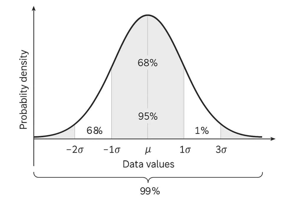
The Empirical Rule applies to a normal distribution curve, a symmetrical bell-shaped curve where data clusters around the mean (average). It states:
68% of data falls within one standard deviation (±1σ) of the mean.
95% falls within two standard deviations (±2σ).
99.7% falls within three standard deviations (±3σ).
This rule leverages the symmetrical bell curve to estimate probabilities, making it a go-to tool for datasets like test scores or heights that follow a normal distribution. The mean and standard deviation define the curve’s center and spread, allowing quick probability calculations.
Step-by-Step: How to Find Probability Using the Empirical Rule
Here’s a beginner-friendly empirical rule step-by-step guide to calculate probability under normal distribution:
Identify Mean (μ) and Standard Deviation (σ):
Find the dataset’s average (μ) and standard deviation (σ). For example, test scores might have μ = 100 and σ = 15.Determine Standard Deviations from the Mean:
Calculate how many standard deviations a value or range is from the mean using the z-score formula:
[ Z = \frac{x – \mu}{\sigma} ]
For a score of 115: ( Z = \frac{115 – 100}{15} = 1 ).Apply Empirical Rule Thresholds:
Within ±1σ: 68% probability.
Within ±2σ: 95% probability.
Within ±3σ: 99.7% probability.
For a z-score of 1, the probability below this score is 50% (mean) + 34% (half of 68%) = 84%.
Interpret the Result:
The probability represents the area under the curve for the specified range. For example, 68% of data lies between ±1σ.
Example: For a score of 85 (z = -1), the probability of a score below 85 is 50% – 34% = 16%. For faster calculations, use our z-score tool .
Example Problem: Find the Probability Between Two Values
Let’s solve a realistic empirical rule example:
Problem: SAT scores have a mean of 1000 and a standard deviation of 200. What’s the probability of a score between 800 and 1200?
Steps:
Calculate Z-Scores:
For 800: ( Z = \frac{800 – 1000}{200} = -1 )
For 1200: ( Z = \frac{1200 – 1000}{200} = 1 )
Apply the Empirical Rule:
The range from -1σ to +1σ covers 68% of the data, so the probability of a score between 800 and 1200 is 68%.Visualize: The bell curve probability shows the shaded area between 800 and 1200, representing 68% of test-takers.
For quick results, use our main statistics calculator to compute this automatically.
When to Use the Empirical Rule for Probability
The Empirical Rule is ideal for:
Normally Distributed Data: Use for datasets like IQ scores, SAT results, or heights that form a normal distribution curve.
Quick Approximations: Perfect when exact z-tables aren’t needed, such as in classroom settings or initial data analysis.
Real-World Scenarios: Common in education (grading), healthcare (medical metrics), and performance testing (standardized tests).
It’s widely used because it’s simple and doesn’t require advanced software. For tail probabilities, try our tail probability tool .
Limitations of the Empirical Rule
While powerful, the Empirical Rule has limits:
-
Normal Distributions Only: It doesn’t apply to skewed or non-normal data. For non-normal data, consider Chebyshev’s theorem.
-
Approximations: Provides rough estimates (e.g., 68% for ±1σ) rather than precise probabilities, unlike z-tables.
-
Large Samples: Works best with large datasets (n > 30) to ensure normality.
For precise calculations or non-normal data, use z-tables or our zone probability tool .
FAQs
The Empirical Rule estimates probabilities in a normal distribution, showing how data spreads within 1, 2, or 3 standard deviations (68%, 95%, 99.7%).
It’s accurate for normally distributed data with large samples but provides approximations, not exact probabilities like a z-table.
No, it’s only reliable for normal distribution curves. For non-normal data, use Chebyshev’s theorem or other methods.
Probability is the likelihood of a value occurring (e.g., 68% within ±1σ), while percentile ranks a value’s position (e.g., 84th percentile for z = 1).
The z-score and empirical rule connect through standard deviations: z = ±1, ±2, ±3 correspond to 68%, 95%, and 99.7% of data.
Conclusion
Learning how to use empirical rule to find probability is a game-changer for understanding probability under normal distribution. This guide’s empirical rule step-by-step approach makes it easy for students, educators, and analysts to estimate probabilities using the 68-95-99.7 rule explained clearly. From SAT scores to medical data, the Empirical Rule simplifies statistical inference with minimal math. Try our probability tool to calculate probabilities instantly, or explore tools like the main statistics calculator , tail probability tool , z-score approximator , or zone probability tool to deepen your stats knowledge.
Check Our Other Tools:
Empirical Rule Graph Generator
Visualize the 68-95-99.7 Rule with a bell curve showing standard deviation intervals. Great for quick insights and presentations.
Try CalculatorBell Curve Generator
Create customizable bell curve plots for any normal distribution. Perfect for data analysis and visual reports.
Standard Deviation Shading Calculator
Shade areas under the curve based on standard deviation. Instantly see data coverage between values.
Try CalculatorZ-Score to Graph Plotter
Plot Z-scores on a bell curve and see where your value lies. Understand percentiles and probabilities at a glance.
Try Calculator