
How to Make a Bell Curve in Excel
Learning how to make a bell curve in excel takes about ten minutes once you know the right formula. A bell curve — also called a normal distribution graph in Excel — is just a set of x values paired with heights from the NORM.DIST function, plotted on a Scatter chart with smooth lines. This guide walks through the whole process with a worked IQ example (mean 100, standard deviation 15), so you can check every number as you go.
Short answer: Use NORM.DIST with FALSE and a Scatter with Smooth Lines chart. Put your mean in B2 and your standard deviation in B3, build x values from three standard deviations below the mean to three above it with =SEQUENCE(61,1,B2-3*B3,B3/10), get the curve heights with =NORM.DIST(D2#,B2,B3,FALSE), then select the two columns and choose Insert → Scatter (X, Y) → Scatter with Smooth Lines.
If you only need the finished picture, skip the spreadsheet entirely: our free bell curve generator draws the same IQ curve in seconds, with data paste and PNG download. The rest of this guide shows the Excel version step by step, so you understand — and can reuse — every formula.
What you need before you start
You need Excel 365 or Excel 2021 for the SEQUENCE version below; any older version works too with the drag-down fallback in Step 1. You also need a mean and a standard deviation — either known values, as in our IQ example, or calculated from your own data with AVERAGE and STDEV.P or STDEV.S (see the section on making a bell curve from your own data below). A normal curve in Excel is nothing more than those two numbers plus the NORM.DIST function, so do not worry about add-ins or extra software.
Set up two settings cells first, because every formula below points at them: type 100 in cell B2 (the mean, μ) and 15 in cell B3 (the standard deviation, σ). Label them in column A — “Mean” in A2 and “Standard deviation” in A3 — so the sheet is easy to read later. Using cells instead of typed numbers means the whole curve updates the moment you change the mean or SD, which is exactly how an Excel bell curve template should behave.
Step 1 — Build the x values (the IQ scores)
Put the column headings in row 1: type “IQ score” in D1 and “Curve height” in E1. Then enter the x values in column D. In modern Excel (365 or 2021), click D2 and type the spill formula =SEQUENCE(61,1,B2-3*B3,B3/10). It fills D2:D62 with 61 values from 55 to 145 in steps of 1.5 — three standard deviations either side of the mean of 100. That range covers 99.7% of a normal distribution, so the curve shows both tails.
In older Excel, or if you want the values as plain numbers instead of a spill range, use the drag-down fallback: in D2 type =B2-3*B3, in D3 type =D2+$B$3/10, then drag D3 down to D62. The dollar signs lock the standard deviation reference so the step stays at 1.5 as you drag. This is how to make a bell curve in Excel without SEQUENCE — the result is identical.
Step 2 — Calculate the curve heights with NORM.DIST
The height of the curve at each x value comes from the NORM.DIST formula for a bell curve. In modern Excel, click E2 and type =NORM.DIST(D2#,B2,B3,FALSE) — the # tells Excel to use the whole spilled range from D2. In older Excel, type =NORM.DIST(D2,$B$2,$B$3,FALSE) in E2 and drag it down to E62. The FALSE at the end is essential: it asks for the probability density (the height of the curve). Use TRUE here and you get a rising S-shaped curve instead — the most common mistake, covered in the fixes table below.
Check your numbers against the verified values in this table before you chart anything. If yours match, your formulas are right:
| IQ score (x) | Distance from the mean | NORM.DIST value |
|---|---|---|
| 100 | 0 (the mean) | 0.0266 (the peak) |
| 115 | +1 SD | 0.0161 |
| 85 | −1 SD | 0.0161 |
| 130 | +2 SD | 0.0036 |
| 70 | −2 SD | 0.0036 |
The curve is symmetric: 85 and 115 give the same height, as do 70 and 130. The peak height of 0.0266 at the mean is the highest point on the whole curve, and the heights fall away quickly — by 130 or 70 the curve is already close to the axis.
Step 3 — Make the chart (Scatter with Smooth Lines)
Select the two columns of data, D1:E62, including the headings. Then go to Insert → Charts → Scatter (X, Y) → Scatter with Smooth Lines. A smooth bell curve appears, peaking at 100 and falling away on both sides. Give the chart a clear title — double-click the chart title and type “IQ Bell Curve (Mean 100, SD 15)” — then remove the legend (click it and press Delete) and label the axes: use Chart Design → Add Chart Element → Axis Titles, with “IQ score” on the horizontal axis and “Density” on the vertical axis.
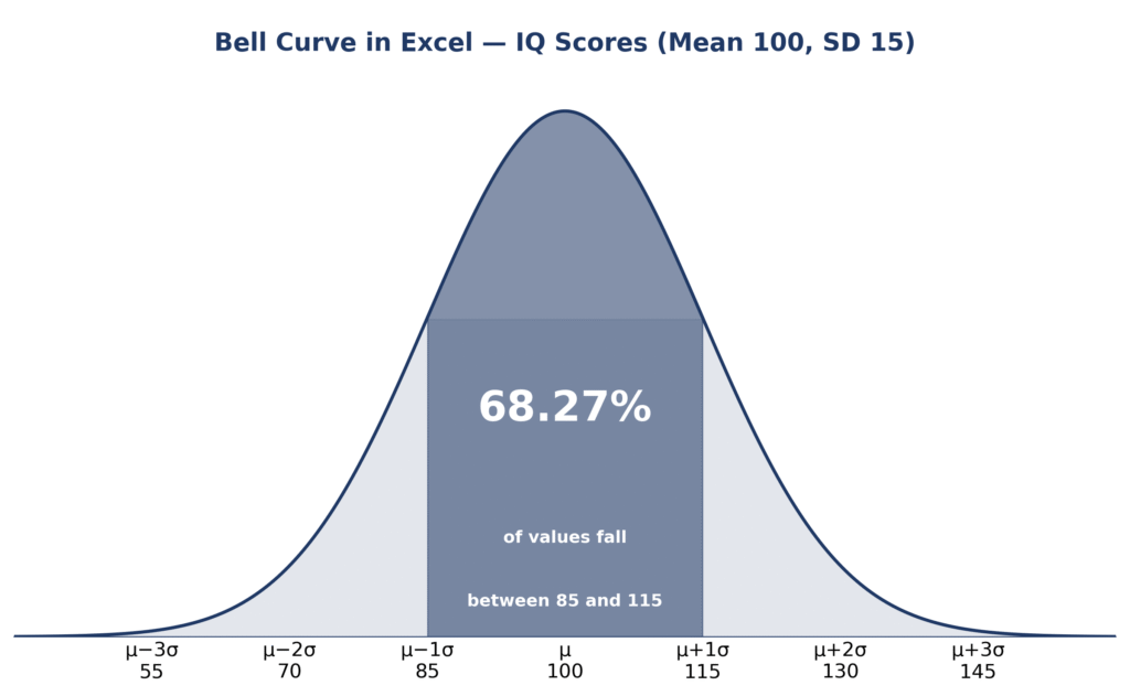
Your scatter chart bell curve should look like the diagram above: one smooth hump, highest at the mean, with both tails nearly touching the axis at 55 and 145. If the shape looks wrong, check the fixes table near the end of this guide before changing anything else.
Markers at each standard deviation make the curve much easier to read. Build a small helper table — for example in columns G and H — with the marker positions −3 to +3 and their scores and heights: the score is μ + kσ, so the markers sit at 55, 70, 85, 100, 115, 130 and 145, and the height at each one is =NORM.DIST(score,100,15,FALSE), giving 0.0003, 0.0036, 0.0161, 0.0266, 0.0161, 0.0036 and 0.0003. (At ±3 SD the height is only 0.0003, which is why the tails look flat.) Right-click the chart, choose Select Data, and add this table as a second series with markers and no connecting line. Then add error bars to that series (Chart Design → Add Chart Element → Error Bars → More Error Bars Options, direction Minus, no cap) and set their length so the bars run from each marker down to the axis. Each bar now marks one standard deviation, and the bar at 100 marks the peak. If you want the z value behind each marker, the free z-score calculator converts any IQ score to its z-score in one step.
Step 4 — Shade the 68.27% band (optional)
To shade the middle of the curve, add a helper column in F: in F2 type =IF((D2#>=85)*(D2#<=115),E2#,0) (or the dragged-down version =IF(AND(D2>=85,D2<=115),E2,0)) and copy it down. The column holds the curve height between 85 and 115 and zero everywhere else. Then change the chart to a combo chart: right-click the chart, choose Change Chart Type → Combo, keep the curve as a Scatter with Smooth Lines, and set the helper series to Area. The middle band fills in, showing the middle 68.27% of the distribution. Check it with the probability formula: =NORM.DIST(115,100,15,TRUE)-NORM.DIST(85,100,15,TRUE) = 0.6827. That is the empirical rule in action — about 68% of IQ scores fall within one standard deviation of the mean, as explained on our empirical rule page.
Step 5 — Probabilities with NORM.DIST(TRUE)
The same NORM.DIST function answers probability questions when you switch the last argument to TRUE — that returns the cumulative probability up to a value. These are the figures for our IQ example, all verified:
| Question | Excel formula | Answer |
|---|---|---|
| P(X < 115) — score below 115 | =NORM.DIST(115,100,15,TRUE) | 0.8413 (84.13%) |
| P(X > 130) — score above 130 | =1-NORM.DIST(130,100,15,TRUE) | 0.0228 (2.28%) |
| P(85 < X < 115) — within 1 SD | =NORM.DIST(115,100,15,TRUE)-NORM.DIST(85,100,15,TRUE) | 0.6827 (68.27%) |
| 90th percentile — score at the 90th percentile | =NORM.INV(0.9,100,15) | 119.22 |
An IQ of 115 sits at about the 84th percentile, an IQ of 130 at about the 98th percentile, and only about 2.28% of people score above 130. To check any of these without Excel, use the normal distribution calculator or the empirical rule percentile calculator with the same mean and SD.
If you have a list of real scores instead of a known mean and SD, start by calculating both from the data. With the scores in column A, use =AVERAGE(A:A) for the mean, =STDEV.P(A:A) if the data is the whole group you care about, and =STDEV.S(A:A) if it is a sample taken from a larger group. The two SD functions give slightly different answers — STDEV.S divides by n−1, STDEV.P by n — so use STDEV.P for a complete class or team and STDEV.S for a sample. If you are unsure which one fits, the standard deviation calculator works out both from the same pasted data. Then put the calculated mean and SD in B2 and B3 and follow Steps 1–3 exactly as above, with the computed numbers instead of 100 and 15.
Common errors and fixes
Almost every failed bell curve comes from one of these six mistakes. Find your symptom, apply the fix, and the curve should appear:
| Problem | What went wrong | Fix |
|---|---|---|
| S-shaped curve | Used TRUE instead of FALSE in NORM.DIST | Change the last argument to FALSE for curve heights |
| #NUM! error | Standard deviation is 0 or negative | Check B3 is a positive number (15 in our example) |
| Flat or lopsided curve | X values cover only one side of the mean | Build x values from mean − 3 SD to mean + 3 SD (55 to 145) |
| Straight lines instead of a curve | Used a Line chart, not a Scatter chart | Re-create the chart as Scatter (X, Y) with Smooth Lines |
| #NAME? error | Typed NORMDIST, or a locale that needs semicolons | Use NORM.DIST with commas — or semicolons if your Excel locale needs them |
| Curve does not update | Typed values instead of formulas, or forgot $ absolute references | Use formulas pointing at B2 and B3, with $ on references you drag down |
Skip Excel — use the free tool instead
If you need the finished curve rather than the spreadsheet practice, the bell curve generator draws the same IQ curve in seconds: enter the mean and standard deviation, paste your data if you have it, and download the graph as a PNG. It is the fastest way to check your Excel result, too — if the tool’s curve and your chart do not match, one of your formulas is off. For a single IQ score, the IQ bell curve calculator shows its percentile on the same curve.
How to create a bell curve in Excel with mean and standard deviation
Put the mean in B2 and the standard deviation in B3, build x values from mean − 3 SD to mean + 3 SD with SEQUENCE (or the drag-down fallback), calculate heights with =NORM.DIST(x, mean, SD, FALSE), and plot the two columns on a Scatter with Smooth Lines chart. That is the whole method — Steps 1–3 above walk through it with the IQ numbers filled in.
Why is my bell curve S-shaped in Excel?
Your curve is S-shaped because the NORM.DIST formula ends in TRUE instead of FALSE. TRUE returns the cumulative probability, which rises from 0 to 1 in an S shape; FALSE returns the probability density, which is the bell shape. Change the last argument to FALSE, and the curve becomes a bell.
How to shade area under a bell curve in Excel
Add a helper column that keeps the curve height only inside the range you want shaded — for the middle band, =IF((D2#>=85)*(D2#<=115),E2#,0) — and zero elsewhere. Then change the chart to a Combo chart with the helper series shown as an Area series, as in Step 4 above. The shaded band covers 68.27% of the curve between 85 and 115.
For the statistical background behind the normal distribution, see the NIST/SEMATECH e-Handbook of Statistical Methods.
Frequently asked questions
What is the NORM.DIST formula for a bell curve?
Use =NORM.DIST(x, mean, standard_dev, FALSE), for example =NORM.DIST(D2,$B$2,$B$3,FALSE) with the mean in B2 and the standard deviation in B3. FALSE returns the curve height (probability density); use TRUE only when you want a cumulative probability.
How do I make a bell curve in Excel from data?
Calculate the mean with =AVERAGE(A:A) and the standard deviation with =STDEV.P(A:A) for a whole group or =STDEV.S(A:A) for a sample, put the results in B2 and B3, then follow Steps 1–3: build the x values, calculate the heights with NORM.DIST, and plot a Scatter chart with Smooth Lines.
Can I make a bell curve in Excel without SEQUENCE?
Yes. In D2 type =B2-3*B3, in D3 type =D2+$B$3/10, drag D3 down to D62, then use =NORM.DIST(D2,$B$2,$B$3,FALSE) in E2 and drag it down. The result is identical to the SEQUENCE version and works in any Excel version.
Is there a free bell curve Excel template?
Yes — the layout in this guide is a reusable template: copy the settings cells (B2 and B3), the SEQUENCE or drag-down x values, and the NORM.DIST column into a blank workbook and save it. Or skip the setup entirely and use the free bell curve generator, which draws the same curve and downloads it as a PNG.
Why is my bell curve flat?
A flat curve usually means the x values cover too narrow a range, or the standard deviation is much larger than the range you plotted. Check that B3 is the real standard deviation (15 in our example) and that the x values run from mean − 3 SD to mean + 3 SD — 55 to 145 for IQ scores.
How do I add standard deviation lines to a bell curve in Excel?
Build a helper table with the scores 55, 70, 85, 100, 115, 130 and 145 and their NORM.DIST heights, add it as a second series with markers and no line, then add Minus error bars to that series running down to the axis. Step 3 above gives the full instructions.
What is the difference between NORM.DIST and NORM.S.DIST?
NORM.DIST takes any mean and standard deviation, while NORM.S.DIST is the standard normal distribution with mean 0 and standard deviation 1. For an IQ curve with mean 100 and SD 15, use NORM.DIST; NORM.S.DIST only works with z-scores.
How do I find the percentage of scores between two values in Excel?
Subtract the two cumulative probabilities: =NORM.DIST(upper, mean, SD, TRUE)-NORM.DIST(lower, mean, SD, TRUE). For IQ scores between 85 and 115, that is =NORM.DIST(115,100,15,TRUE)-NORM.DIST(85,100,15,TRUE) = 0.6827, or 68.27%.
Check Tools
Try these free tools to check your Excel work or skip the spreadsheet altogether:
Bell Curve Generator
Draw a bell curve from any mean and SD and download it as a PNG.
ToolsTry Calculator → ● LiveZ-Score Calculator
Turn any value into a z-score, percentile and probability.
ToolsTry Calculator → ● LiveNormal Distribution Calculator
Find CDF, inverse and graph values for any normal distribution.
ToolsTry Calculator → ● LiveStandard Deviation Calculator
Work out the mean, variance and standard deviation from pasted data.
ToolsTry Calculator → ● LiveIQ Bell Curve Calculator
See where any IQ score sits on the bell curve.
ToolsTry Calculator → ● LiveEmpirical Rule Percentile Calculator
Convert percentiles to values with a mean and SD.
ToolsTry Calculator → ● LiveExplore All Statistical Tools
Browse every free calculator on this site.
ToolsTry Calculator →