These normal distribution examples show how the bell curve works in real life — with a mean, a standard deviation, and an exact probability for every case. Heights, IQ scores, SAT scores, birth weights, blood pressure, and even bolt diameters all follow, approximately, the same smooth, symmetric shape. Below, each of the 12 examples of normal distribution in statistics is worked out with a z-score, so you can see the answer and check it yourself in our free calculator.
Why do so many different things look the same? Because each one is the sum of many small, independent influences — genes, nutrition, practice, tiny manufacturing variations — and the central limit theorem says that kind of sum piles up into a bell curve. That is why normal distribution probability examples like the ones below are useful far beyond the textbook: the same method answers questions about test scores, health measurements, and factory quality control.
Unlike our applications of the empirical rule page, which uses the 68-95-99.7 approximations, this page gives exact probabilities from the normal curve. For the theory behind the curve, see the NIST/SEMATECH e-Handbook of Statistical Methods.
How to Solve Normal Distribution Problems
Every example below follows the same four steps. Learn them once, and you can solve any normal distribution problem.
- Find the mean (μ) and standard deviation (σ). These two numbers describe the whole distribution: μ is the center, and σ is the spread.
- Convert the value to a z-score. Use z = (x − μ) / σ. The z-score says how many standard deviations a value sits from the mean.
- Look up the probability. Use a z-table or a calculator to turn the z-score into a probability or percentile. If you need a refresher, see how to calculate a z-score and how to read a z-table.
- Interpret the result. Turn the decimal back into a percentage and a plain-English sentence: for example, “about 16 out of 100 men are taller than 73 inches.”
A quick check: the 68-95-99.7 rule says about 68.27% of values fall within one standard deviation of the mean, 95.45% within two, and 99.73% within three. You can see the same pattern in the normal distribution and the empirical rule guide.
What Are Some Examples of Normal Distribution?
Short answer: men’s heights, IQ scores, SAT and ACT scores, birth weights, blood pressure, and manufactured parts are classic real life examples of normal distribution. The 12 worked examples below cover biology, test scores, health, manufacturing, and everyday life — each with its mean, standard deviation, z-score, and exact probability.
Normal Distribution Examples in Biology
Biology is full of bell curves, because a measurement like height is shaped by hundreds of genes plus nutrition, health, and environment. No single factor dominates, so values cluster near the average and thin out toward the extremes — the classic normal distribution in real life.
Example 1 — Men’s Heights
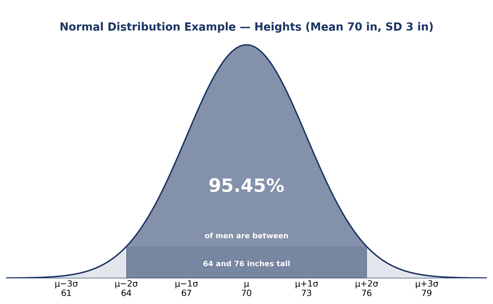
Adult men’s heights are approximately normal with mean μ = 70 inches and standard deviation σ = 3 inches. What percentage of men are between 64 and 76 inches tall?
Convert each end to a z-score: z = (64 − 70) / 3 = −2.00 and z = (76 − 70) / 3 = +2.00. The area between z = −2 and z = +2 is 95.45%, so P(64 < X < 76) = 95.45%. The same method gives P(X > 73): z = (73 − 70) / 3 = +1.00, and the area above z = +1 is 15.87%. In other words, about 16 in 100 men are taller than 73 inches. Check it yourself in the Normal Distribution Calculator.
You can draw the same curve for any mean and spread with the Bell Curve Generator.
Normal Distribution Example: Test Scores
Standardized tests are designed to be bell-shaped: most students score near the middle, and very high or very low scores are rare. That makes test scores the most familiar bell curve examples in statistics classes.
Example 2 — IQ Scores
IQ scores are approximately normal with mean μ = 100 and standard deviation σ = 15. What percentage of people score between 85 and 115? z = (85 − 100) / 15 = −1.00 and z = (115 − 100) / 15 = +1.00, so P(85 < X < 115) = 68.27%. And a score above 130? z = (130 − 100) / 15 = +2.00, so P(X > 130) = 2.28% — about 2 people in 100. Check the IQ probabilities in the calculator.
Example 3 — SAT Scores
SAT scores are approximately normal with mean μ = 500 and standard deviation σ = 100. What is the probability of scoring above 600? z = (600 − 500) / 100 = +1.00, so P(X > 600) = 15.87%. Between 400 and 600, z runs from −1 to +1, so P(400 < X < 600) = 68.27%. Verify the SAT numbers yourself.
Example 4 — ACT Scores
ACT scores are approximately normal with mean μ = 21 and standard deviation σ = 5. A student scores 26. What percentile is that? z = (26 − 21) / 5 = +1.00, and Φ(1.00) = 0.8413, so the score is at the 84.13th percentile — higher than about 84% of test-takers. You can also plot the z-score on a bell curve to see where 26 sits. Check the ACT percentile in the Normal Distribution Calculator.
Normal Distribution Examples in Biology
Example 5 — Birth Weight
Birth weights are approximately normal with mean μ = 7.5 pounds and standard deviation σ = 1.0 pound. What share of newborns weigh between 6.5 and 8.5 pounds? z = (6.5 − 7.5) / 1.0 = −1.00 and z = (8.5 − 7.5) / 1.0 = +1.00, so P(6.5 < X < 8.5) = 68.27%. About two-thirds of babies fall in that one-pound band around the mean. Run the birth-weight numbers yourself.
Normal Distribution Examples in Health and Manufacturing
Doctors use bell curves to define healthy ranges, and factories use them to keep parts within tolerance. In both cases the same idea applies: most values sit near the mean, and the standard deviation sets what counts as unusual.
Example 6 — Systolic Blood Pressure
Systolic blood pressure is approximately normal with mean μ = 120 mmHg and standard deviation σ = 12 mmHg. What is the probability that a randomly chosen adult has a reading above 132? z = (132 − 120) / 12 = +1.00, so P(X > 132) = 15.87%. Between 108 and 132, z runs from −1 to +1, so P(108 < X < 132) = 68.27%. Check the blood-pressure probabilities in the calculator.
Example 7 — Bolt Diameter
A machine makes bolts whose diameters are approximately normal with mean μ = 10.00 mm and standard deviation σ = 0.05 mm. What percentage of bolts measure between 9.90 mm and 10.10 mm? z = (9.90 − 10.00) / 0.05 = −2.00 and z = (10.10 − 10.00) / 0.05 = +2.00, so P(9.90 < X < 10.10) = 95.45%. A bolt wider than 10.05 mm has z = +1.00, so P(X > 10.05) = 15.87%. Verify the bolt measurements yourself.
Example 8 — Light-Bulb Service Requests
A store receives light-bulb service requests that are approximately normal with mean μ = 59 per week and standard deviation σ = 9. What is the probability of more than 68 requests in a week? z = (68 − 59) / 9 = +1.00, so P(X > 68) = 15.87%. Between 50 and 68 requests, z runs from −1 to +1, so P(50 < X < 68) = 68.27%. Check the service-request probabilities in the calculator.
Example 9 — Car Service Time
The time to service a car is approximately normal with mean μ = 41 minutes and standard deviation σ = 5 minutes. What is the probability a service takes more than 46 minutes? z = (46 − 41) / 5 = +1.00, so P(X > 46) = 15.87%. Between 36 and 46 minutes, z runs from −1 to +1, so P(36 < X < 46) = 68.27%. Run the car-service numbers yourself.
Example 10 — Candy Bags
Bags of candy contain a number of candies that is approximately normal with mean μ = 57.3 and standard deviation σ = 1.2. What is the probability that a bag has fewer than 55 candies? z = (55 − 57.3) / 1.2 = −1.92. From the z-table, Φ(−1.92) = 0.0274, so P(X < 55) = 2.74%. Fewer than 3 bags in 100 are that short. You can plot the 68-95-99.7 bands for this distribution with the Empirical Rule Graph Generator. Check the candy-bag probability in the calculator.
Normal Distribution Examples in Biology
Example 11 — Iguana Mass
The masses of a population of iguanas are approximately normal with mean μ = 950 grams and standard deviation σ = 325 grams. What is the probability that a randomly chosen iguana weighs less than 400 grams? z = (400 − 950) / 325 = −1.69. From the z-table, Φ(−1.69) = 0.0455, so P(X < 400) = 4.55%. Only about 1 iguana in 22 is that light. Verify the iguana probability in the calculator.
Example 12 — Cecil’s Height
Cecil’s height is at the 73rd percentile of a group whose heights are normal with mean μ = 152.9 cm and standard deviation σ = 8.5 cm. How tall is Cecil? The 73rd percentile corresponds to z ≈ +0.61, so x = μ + zσ = 152.9 + 0.61 × 8.5 = 158.1 cm. Working backwards from a percentile to a value is called an inverse normal problem — you can also find percentiles with the Empirical Rule Percentile Calculator. Check Cecil’s height in the Normal Distribution Calculator.
Normal Distribution Examples in Everyday Life
Beyond the textbook, normal distribution examples in everyday life are everywhere: the time a morning commute takes, the weight of apples in a bag, the amount of coffee a cafe serves in a day, and the scores on a class test. Each one is the result of many small, unrelated factors adding up, so most days look ordinary and extreme days are rare. The same z-score method from the examples above works for any of them — as long as the data is roughly bell-shaped.
Is IQ Normally Distributed?
Yes, approximately — and partly by design. Modern IQ tests are scored so the population mean is 100 and the standard deviation is 15, and the raw scores are transformed to fit a bell curve. That is why the IQ example above works so cleanly: about 68.27% of people score between 85 and 115, and only about 2.28% score above 130. In practice, real IQ distributions have slightly heavier tails than a perfect bell curve, and scores can shift with education and test design, so “normal” is a good model, not a law of nature.
When Is Data Not Normally Distributed?
The normal model fails whenever the bell shape breaks down. Skewed data — such as household income, where a few very high values stretch one tail — is not symmetric. Bounded data — such as test scores capped at 100, or waiting times that cannot go below zero — piles up at a boundary instead of tapering off. Bimodal data — such as the heights of men and women mixed together — has two peaks, not one. And small samples may look lumpy or irregular even when the underlying population is normal. Always plot your data — a histogram or a bell curve — before assuming it is normal: if the shape is not a bell, the probabilities on this page do not apply.
When the data is roughly normal, the method is always the same: find μ and σ, convert to a z-score, look up the probability, and interpret it — then check it yourself in the Normal Distribution Calculator.
Frequently Asked Questions About Normal Distribution Examples
Where can I find normal distribution examples with solutions?
Right here: the 12 examples above are each worked out step by step, with the mean, standard deviation, z-score, and exact probability. Start with the men’s heights example (μ = 70 inches, σ = 3 inches), then try the IQ, SAT, and blood pressure examples — and check every answer in the Normal Distribution Calculator.
What is a normal distribution example with heights?
Men’s heights are the classic example: they are approximately normal with mean μ = 70 inches and standard deviation σ = 3 inches. About 95.45% of men are between 64 and 76 inches tall, and 15.87% are taller than 73 inches.
What is a normal distribution example with test scores?
SAT scores are approximately normal with mean μ = 500 and standard deviation σ = 100: 15.87% of students score above 600. ACT scores (μ = 21, σ = 5) work the same way — a score of 26 is at the 84.13th percentile.
What is the most common example of a normal distribution?
Human height is the most common example, followed by IQ scores and standardized test scores. All three are shaped by many small, independent factors, which is why they pile up into a bell curve around the average.
How do you find the probability in a normal distribution?
Find the mean (μ) and standard deviation (σ), convert the value to a z-score with z = (x − μ) / σ, then look up the z-score in a z-table or enter it in a normal distribution calculator to get the probability.
What percentage is within 1, 2, and 3 standard deviations?
About 68.27% of values fall within 1 standard deviation of the mean, 95.45% within 2, and 99.73% within 3. This is the empirical rule, or 68-95-99.7 rule.
Can a normal distribution be skewed?
No. A normal distribution is symmetric by definition, with the mean, median, and mode all equal. If data is skewed — like household income — it is not normally distributed, and normal probabilities do not apply to it.
Why is the normal distribution important?
Because so many real measurements are approximately normal, and because the central limit theorem says averages of many small effects pile up into a bell curve. It is the foundation for z-scores, percentiles, confidence intervals, and hypothesis tests.
Check Tools
Put the examples above into practice with these free tools.
Normal Distribution Calculator
Find exact probabilities, percentiles, and z-scores for any normal distribution — check every example on this page.
ToolsTry Calculator → ● LiveBell Curve Generator
Draw a bell curve for any mean and standard deviation and see the 68-95-99.7 bands.
ToolsTry Calculator → ● LiveZ-Score Calculator
Convert any value to a z-score and find its percentile and probability in one step.
ToolsTry Calculator → ● LiveZ-Score Graph Plotter
Plot a z-score on a bell curve to see exactly where a value sits in the distribution.
ToolsTry Calculator → ● LiveEmpirical Rule Percentile Calculator
Find the percentile for a value, or the value for a percentile, from a mean and standard deviation.
ToolsTry Calculator → ● LiveExplore All Statistical Tools
Browse the full set of free statistics calculators and generators in one place.
ToolsTry Calculator →Check Articles
What is the Empirical Rule?
The 68.27%, 95.45% and 99.73% shares explained from the start.
ArticleRead Article → ● LiveNormal Distribution and the Empirical Rule
How the bell curve works, and why it makes the rule possible.
ArticleRead Article → ● LiveHow to Use Empirical Rule Calculator
Worked steps for the calculator, from mean and standard deviation to results.
ArticleRead Article → ● LiveReal-Life Applications of Percentiles in Normal Distribution
Real-life applications of percentiles in normal distribution turn a score into a rank.
ArticleRead Article → ● LiveEmpirical Rule vs. Confidence Intervals: What’s the Difference?
The empirical rule and the confidence interval are not the same thing.
ArticleRead Article → ● LiveHow to Calculate a Z-Score
A z-score tells you how many standard deviations a value sits from the mean.
ArticleRead Article → ● LiveHow to Read a Z-Table
A z-table is a reference table that gives the area under the standard normal curve to the left of a given z-score.
ArticleRead Article →