
Chebyshev's Theorem Explained
Chebyshev’s theorem gives you a guaranteed minimum for any dataset — no matter how skewed, lumpy or strange its shape. If you know the mean and the standard deviation, you already know that at least 75% of the values sit within two standard deviations of the mean.
Chebyshev’s theorem says that for any dataset, whatever its shape, at least 1 − 1/k² of the values lie within k standard deviations of the mean. It is a floor, not an estimate: the real share is always at least that large, and usually much larger. That guarantee is what separates it from the empirical rule, which only applies to bell-shaped data.
Chebyshev’s theorem guarantees that, for any dataset whatever its shape, at least 1 − 1/k² of the values lie within k standard deviations of the mean. For k = 2 that is at least 75%, and for k = 3 at least 88.89%.
What Is Chebyshev’s Theorem?
Chebyshev’s theorem is a guarantee about any set of numbers: at least a fixed share of the values must lie within a given number of standard deviations of the mean — and it holds without knowing anything about the shape of the data. The data can be bell-shaped, skewed like incomes, split into two humps, or flat like a die roll: the guarantee holds all the same.
It is named after Pafnuty Chebyshev, a Russian mathematician of the 1800s who proved that a mean and a standard deviation are enough to put a floor under any distribution. Most statistical rules tell you what usually happens; this one tells you what must happen, at minimum. The wording matters: the theorem says “at least” — 75% and 88.89% are minimums, not predictions. In practice the real share is usually much larger. To see how the two rules compare, read the empirical rule vs Chebyshev’s theorem guide, or check a result with the Chebyshev’s theorem calculator. The definitions here follow the NIST/SEMATECH e-Handbook of Statistical Methods.
The Formula: 1 − 1/k²
For any number k greater than 1, at least (1 − 1/k²) × 100% of the values lie within k standard deviations of the mean — in the interval from μ − kσ to μ + kσ, where μ is the mean and σ is the standard deviation. The k is yours to choose: k = 2 looks two standard deviations each side, k = 3 looks three.
Put k = 2 in and you get 1 − 1/4 = 3/4, or 75%. Put k = 3 in and you get 1 − 1/9 = 8/9, or 88.89%. The guarantee grows as k grows but never reaches 100%: even at k = 10 it only promises 99%. That is the price of assuming nothing.
| k (standard deviations) | Interval | Minimum share inside |
|---|---|---|
| 1.5 | μ ± 1.5σ | 55.56% |
| 2 | μ ± 2σ | 75% |
| 2.5 | μ ± 2.5σ | 84% |
| 3 | μ ± 3σ | 88.89% |
| 4 | μ ± 4σ | 93.75% |
| 5 | μ ± 5σ | 96% |
| 10 | μ ± 10σ | 99% |
Read the table the other way round and it gives the maximum share outside the band: at most 1/k² of the values lie beyond k standard deviations — at most 25% outside two, at most 11.11% outside three. That “at most” form is Chebyshev’s inequality, the form you meet in probability courses. You need a standard deviation first: see how to calculate standard deviation.
Worked Example: Heights
Take heights with a mean of 60 inches and a standard deviation of 8 inches. The working is the same every time: the interval is μ ± kσ, and the guaranteed share is 1 − 1/k².
| k | Interval | At least this share inside |
|---|---|---|
| 1.5 | 60 ± 12, that is [48, 72] | 55.56% |
| 2 | 60 ± 16, that is [44, 76] | 75% |
| 3 | 60 ± 24, that is [36, 84] | 88.89% |
| 4 | 60 ± 32, that is [28, 92] | 93.75% |
Read the k = 2 row aloud: at least 75% of the heights lie between 44 and 76 inches. The theorem does not say the heights are normally distributed, and it does not care whether they are. If they happened to be bell-shaped, the real share inside [44, 76] would be about 95.45% — well above the guaranteed 75%. The guarantee is the floor, not the forecast.
Try it yourself: enter a mean of 60 and a standard deviation of 8 in the Chebyshev’s theorem calculator, then try the numbers for each k in the table above.
The Same Data, Two Answers: Chebyshev vs the Empirical Rule
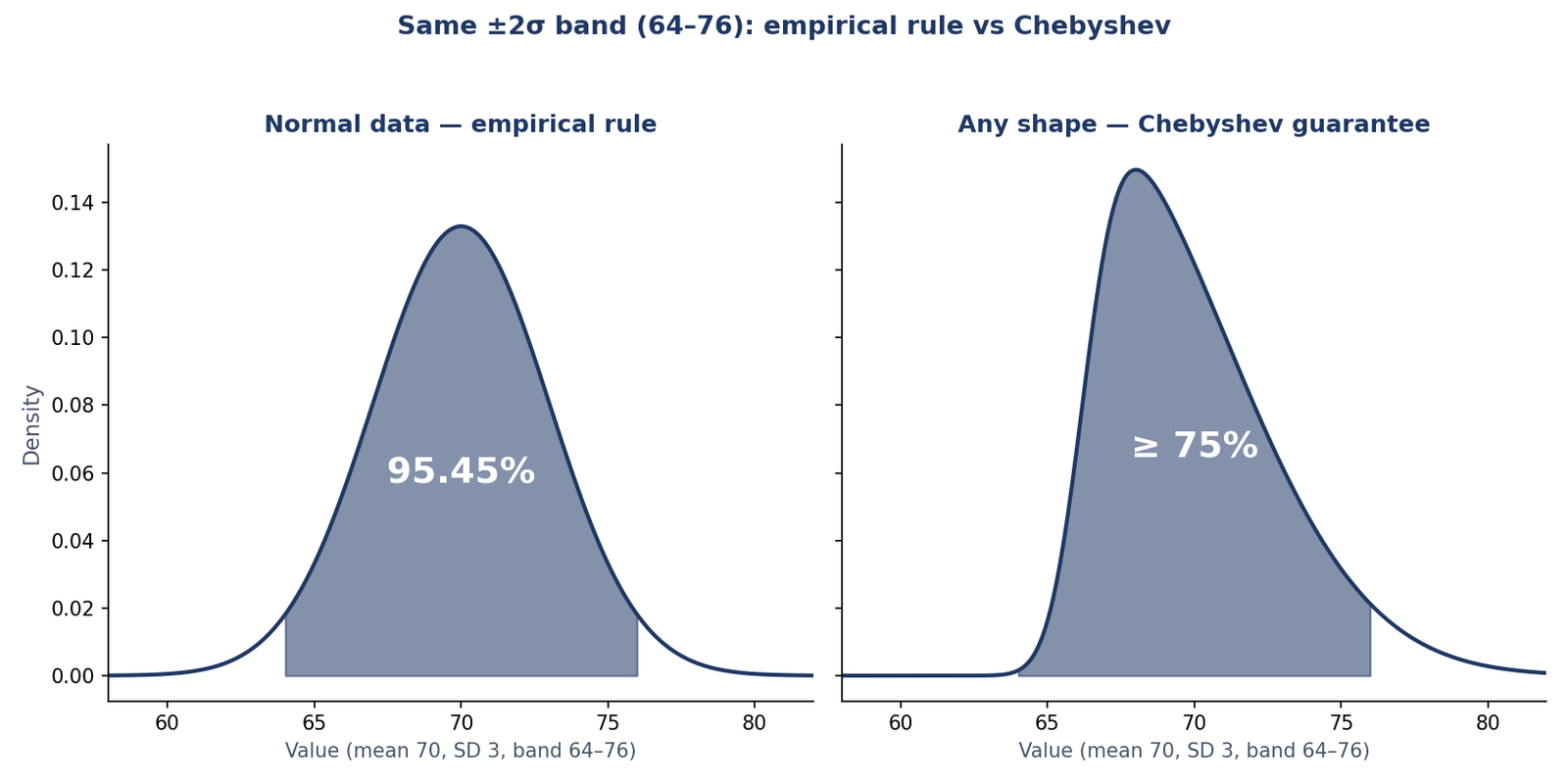
Judge the same heights both ways. Take a group with a mean height of 70 inches and a standard deviation of 3 inches, and look at the band two standard deviations each side: [64, 76].
The empirical rule says 95.45% of the heights fall inside [64, 76] — but only if the heights are normally distributed. Chebyshev’s theorem says at least 75% fall inside [64, 76] — for any shape at all. The diagram at the top of this guide shows both panels side by side: the same band, the same mean and standard deviation, two very different promises.
The difference is the price of the assumption. The empirical rule assumes the bell shape and gives a tight, exact figure. Chebyshev assumes nothing and gives a looser, guaranteed one. If you know the data is normal, use the empirical rule. If you do not know the shape, or it is not normal, 95.45% is a guess and 75% is the only figure you can stand behind. For the full comparison, read empirical rule vs Chebyshev’s theorem — and if your data is bell-shaped, the empirical rule is the guide to reach for.
Real Data: Textbook Costs
Real data is messier than round numbers — and it is where the gap between the guarantee and reality shows up most clearly. Take the textbook costs of 20 students from an OpenStax statistics textbook: the mean cost is $445, and the population standard deviation is $113.91.
For k = 2, the interval is 445 ± 2 × 113.91 = 445 ± 227.82, or [$217.18, $672.82]. The theorem guarantees at least 75% of the 20 costs — at least 15 of them — fall inside.
In fact, 18 of the 20 costs (90%) fall inside — far above the guaranteed 75%. The guarantee was never a prediction of 75%; it was a floor. The two costs outside are the expensive outliers that pull the standard deviation up, and the theorem’s job is to promise something even in their presence. For skewed data like prices, the mean and the median can tell different stories — see mean vs median vs mode if you are choosing which average to report.
Finding k for a Demanded Guarantee
Often the question runs the other way: you want a particular guarantee, and you need the k that delivers it. Solve 1 − 1/k² = p for k and you get k = 1/√(1 − p), where p is the share you want to guarantee as a decimal.
To guarantee at least 90%, set p = 0.90: k = 1/√(1 − 0.90) = 1/√0.10 = 3.16, so the interval is μ ± 3.16σ. To guarantee 95%, k = 1/√0.05 = 4.47; to guarantee 99%, k = 1/√0.01 = 10.
| Guarantee wanted | k needed | Interval |
|---|---|---|
| At least 90% | 3.16 | μ ± 3.16σ |
| At least 95% | 4.47 | μ ± 4.47σ |
| At least 99% | 10 | μ ± 10σ |
The price of a high guarantee is a wide interval. Guaranteeing 99% means going ten standard deviations each side — a band so wide it says very little. A guarantee you can defend costs you precision. Before you solve for k, get σ for your own data with the standard deviation calculator.
When Should I Use Chebyshev’s Theorem Instead of the Empirical Rule?
Use Chebyshev whenever you cannot vouch for the shape of your data. That covers most real-world data: incomes, house prices, waiting times and test scores are skewed or lumpy in ways a bell curve cannot describe, and a small sample gives you no reliable way to check the shape. There the empirical rule’s 68.27%, 95.45% and 99.73% are guesses dressed up as facts, and Chebyshev’s “at least” figures are the only honest ones.
Use the empirical rule when the data is approximately normal — when a histogram shows the familiar bell shape, or the quantity is known to be normal, like measurement error. Then it is the sharper tool: 95.45% inside two standard deviations, where Chebyshev can only promise 75%. A quick check for skew helps you decide: see what is skewness and kurtosis. And if the data is normal and you want exact probabilities, the empirical rule probability finder does the calculation. Short version: normal data → the empirical rule; anything else, or unknown → Chebyshev.
Why Does k = 1 Give 0%?
Put k = 1 into the formula and you get 1 − 1/1² = 1 − 1 = 0. Within one standard deviation, Chebyshev’s theorem guarantees nothing at all. That is the honest consequence of assuming nothing about the shape.
Here is why: a distribution can place half its values exactly at μ − σ and half exactly at μ + σ. Then nothing lies strictly inside one standard deviation, and no theorem that knows only the mean and the standard deviation can rule that out. The guarantee is 0% because the worst case really is that empty. In practice most values do sit within one standard deviation — for bell-shaped data it is 68.27% — but the theorem cannot promise it. It starts saying something useful just above k = 1: k = 1.5 already guarantees 55.56%. Values outside the band are not automatically mistakes — see how to find outliers using IQR before you drop one.
Is Chebyshev’s Theorem the Same as Chebyshev’s Inequality?
Yes — two names for the same result. “Chebyshev’s inequality” is the mathematical form, usually written P(|X − μ| ≥ kσ) ≤ 1/k²: the probability that a value sits k or more standard deviations from the mean is at most 1/k². “Chebyshev’s theorem” is the statistics-textbook name for the same fact as a guarantee: at least 1 − 1/k² of the values lie within k standard deviations.
The two forms say the same thing from opposite sides. The inequality talks about the outside — how much can escape the band. The theorem talks about the inside — how much must stay in it. If at most 25% can sit outside two standard deviations, at least 75% must sit inside. Like the central limit theorem explained in our companion guide, it is a named result you will meet in every statistics course.
Watch the Endpoints: The Income Example
Chebyshev intervals are built from the mean and the standard deviation alone, and neither knows what the quantity can and cannot be. That can produce endpoints that are impossible in the real world.
Take incomes with a mean of $60,000 and a standard deviation of $20,000. For k = 2, at least 75% earn between $20,000 and $100,000. For k = 3, at least 88.89% earn between $0 and $120,000. The lower end of that second interval is exactly $0 — and nobody earns a negative income, so the true lower bound cannot go below zero.
That is not a mistake in the theorem. It does not know incomes cannot be negative; it only knows the mean and the standard deviation, and it draws the widest interval consistent with those two numbers. So sanity-check every endpoint against what the quantity can be. If a bound is impossible, the guarantee still holds — but the useful information is mostly in the other end. A wide, honest interval is still better than a narrow, invented one.
Frequently Asked Questions
What is Chebyshev’s theorem in simple terms?
For any dataset, at least 1 − 1/k² of the values lie within k standard deviations of the mean. For k = 2, at least 75% of values are within two standard deviations; for k = 3, at least 88.89%.
What is the formula for Chebyshev’s theorem?
At least (1 − 1/k²) × 100% of the values lie in the interval [μ − kσ, μ + kσ], where μ is the mean, σ is the standard deviation and k is the number of standard deviations (k > 1).
What is k in Chebyshev’s theorem?
k is how many standard deviations from the mean you are looking at. k = 2 means two standard deviations each side; k = 3 means three. k must be greater than 1 — at k = 1 the theorem guarantees 0%.
When do I use Chebyshev’s theorem instead of the empirical rule?
Use Chebyshev when you do not know the shape of your data, or when it is clearly not normal. Use the empirical rule only when the data is (approximately) normal, because it gives the tighter 68.27%, 95.45% and 99.73% figures.
Why does k = 1 guarantee nothing?
Because 1 − 1/1² = 0. The theorem’s guarantee is 0% within one standard deviation. In practice most values are there, but the theorem — which assumes nothing about the shape — cannot promise it.
Is Chebyshev’s theorem the same as Chebyshev’s inequality?
Yes. They are two names for the same result. “Chebyshev’s inequality” is the mathematical form (P(|X − μ| ≥ kσ) ≤ 1/k²); “Chebyshev’s theorem” is the statistics-textbook name for the same guarantee.
Can Chebyshev’s theorem be used for normal distributions?
Yes, it applies to normal data too — but it is weaker than the empirical rule there. For normal data Chebyshev guarantees at least 75% within two standard deviations, while the empirical rule gives the exact 95.45%.
What is the minimum percentage within 2 standard deviations?
At least 75%. That is the k = 2 case: 1 − 1/2² = 1 − 1/4 = 0.75. Whatever the shape of the data, at least three quarters of the values lie within two standard deviations of the mean.
Check Tools
Try the numbers from this guide with the site’s free calculators:
Chebyshev’s Theorem Calculator
Enter any mean and standard deviation and see the guaranteed minimum percentage inside any number of standard deviations.
Try the Chebyshev’s theorem calculator →
Empirical Rule Probability Finder
For bell-shaped data, get the exact probabilities the empirical rule only approximates.
Try the empirical rule probability finder →
Standard Deviation Calculator
Find σ for your own data set before you apply the theorem.
Try the Standard Deviation Calculator →
Explore All Statistical Tools
See every calculator on the site in one place.
Check Articles
Go deeper with these guides:
Empirical Rule vs Chebyshev’s Theorem
The same data judged both ways, so you can see exactly when each rule wins.
What Is the Empirical Rule
The 68-95-99.7 rule for bell-shaped data, explained from scratch.
How to Calculate Standard Deviation
Work out σ step by step, the number every Chebyshev interval depends on.
Central Limit Theorem Explained
Why sample means form a bell curve, whatever the population looks like.