Standard Normal Distribution

The standard normal distribution is the one normal distribution every other normal distribution can be turned into. It is a bell-shaped curve with a mean of 0 and a standard deviation of 1, written Z ~ N(0, 1). Once a value has been converted to a z-score, a single table — the standard normal table — gives its probability, no matter what the original mean and standard deviation were. That is why the standard normal distribution sits at the centre of z-scores, percentiles, hypothesis tests and confidence intervals, and why learning it once pays off in every statistics course.

In this guide you will learn what the standard normal distribution is, why statisticians standardize, how to convert any normal value with Z = (X − μ) / σ, how to read Φ(z) probabilities from a table, and how to work backwards from a probability to a z-score. Every worked example is checked against the z-table, and the practice problems at the end come with answers.

A standard normal distribution is a normal distribution with mean μ = 0 and standard deviation σ = 1. Its random variable is usually called Z, and the distribution is written Z ~ N(0, 1). The standard normal curve is the familiar bell curve, centred at 0, with most of its area close to the centre and thin tails stretching out on both sides. The z-distribution is simply another name for the same distribution: the distribution of z-scores.

Because the mean is 0, the curve is centred on the origin. Because the standard deviation is 1, one unit on the horizontal axis is one standard deviation. A standard normal random variable Z therefore measures distance from the centre in standard-deviation units: Z = +1 is one standard deviation above the mean, Z = −2 is two standard deviations below it, and Z = 0 is exactly at the mean.

The total area under the standard normal curve is 1, so areas under the curve are probabilities. The notation Φ(z), read “phi of z”, is the cumulative probability up to z:

Φ(z) = P(Z ≤ z)

For example, Φ(0) = 0.5000, because half the area lies to the left of the centre, and Φ(1.00) = 0.8413, because 84.13% of the area lies to the left of z = +1. The phi notation is used throughout this page, and in most textbooks, for exactly this left-tail area.

Properties of the Standard Normal Distribution

• Mean: μ = 0
• Median: 0 — the curve is symmetric, so half the area lies on each side of 0
• Mode: 0 — the peak of the curve is at the centre
• Standard deviation: σ = 1
• Variance: σ² = 1
• Shape: symmetric and bell-shaped, with the mean, median and mode all equal
• Total area: 1, so every area under the curve is a probability between 0 and 1
• Range: z-scores can in principle run from −∞ to +∞, although values beyond ±3 are rare

These properties are what make the standard normal distribution a reference distribution: every normal distribution, whatever its own mean and spread, can be rescaled to look exactly like it.

The mean and standard deviation of the standard normal distribution are fixed by definition: the mean is 0 and the standard deviation is 1. That is the whole point of standardizing. An ordinary normal distribution might have a mean of 100 and a standard deviation of 15, like IQ scores, or a mean of 70 inches and a standard deviation of 3 inches, like men’s heights. After standardization, both become Z ~ N(0, 1), and both are read from the same table.

Short answer: the standard normal distribution has mean μ = 0 and standard deviation σ = 1, so its variance is also 1. If a distribution does not have mean 0 and standard deviation 1, it is a normal distribution, but it is not the standard normal distribution — until you standardize it.

Why Standardize a Normal Distribution?

Without standardization, every normal distribution would need its own probability table: one for IQ scores, one for heights, one for test scores, and so on. Standardizing replaces all of those tables with one. The idea is a simple shift and scale. Subtracting the mean μ shifts the whole curve so its centre sits at 0. Dividing by the standard deviation σ squeezes or stretches the curve so its spread is exactly 1. The shape stays normal; only the centre and the scale change.

Standardizing also makes different measurements comparable. An IQ of 130 and a test score of 85 come from different scales, but as z-scores — +2.00 and +1.50 — they can be compared directly: the IQ score is further above its mean, in standard-deviation units, than the test score is above its mean. That comparison is the job of a z-score calculator, and you can see the same idea worked through in our normal distribution examples.

To standardize a normal distribution, convert each value X to a z-score with the conversion formula:

Z = (X − μ) / σ

Follow these four steps:

1. Find the mean and standard deviation of the normal distribution.
2. Subtract the mean from the value you want to convert.
3. Divide the result by the standard deviation.
4. Look up the resulting z-score in a standard normal table or a calculator to find the probability.

For example, a test score of X = 85 from a distribution with μ = 70 and σ = 10 becomes Z = (85 − 70) / 10 = 15 / 10 = +1.50. The score is 1.50 standard deviations above the mean, and Φ(1.50) = 0.9332, so it sits at the 93.32nd percentile. You can check the arithmetic with our Normal Distribution Calculator, or read the full method in how to calculate a z-score.

The 68-95-99.7 Rule for the Standard Normal Distribution

Because the standard normal distribution has mean 0 and standard deviation 1, the empirical rule takes its simplest form: the intervals are just −1 to +1, −2 to +2 and −3 to +3. The exact percentages, which round to 68, 95 and 99.7, are 68.27%, 95.45% and 99.73%.

Interval (z-scores)	Percentage of the area	Exact value
−1 < Z < +1	About 68%	68.27%
−2 < Z < +2	About 95%	95.45%
−3 < Z < +3	About 99.7%	99.73%

So about two-thirds of all z-scores fall between −1 and +1, about 19 in 20 fall between −2 and +2, and only about 0.27% fall outside ±3. For the full story, including the approximations behind these numbers, see our guide to the normal distribution and the empirical rule.

Each example below starts from a z-score, reads Φ(z) from the standard normal table, and turns the decimal into a percentage and a plain-English sentence. All values have been checked against the z-table.

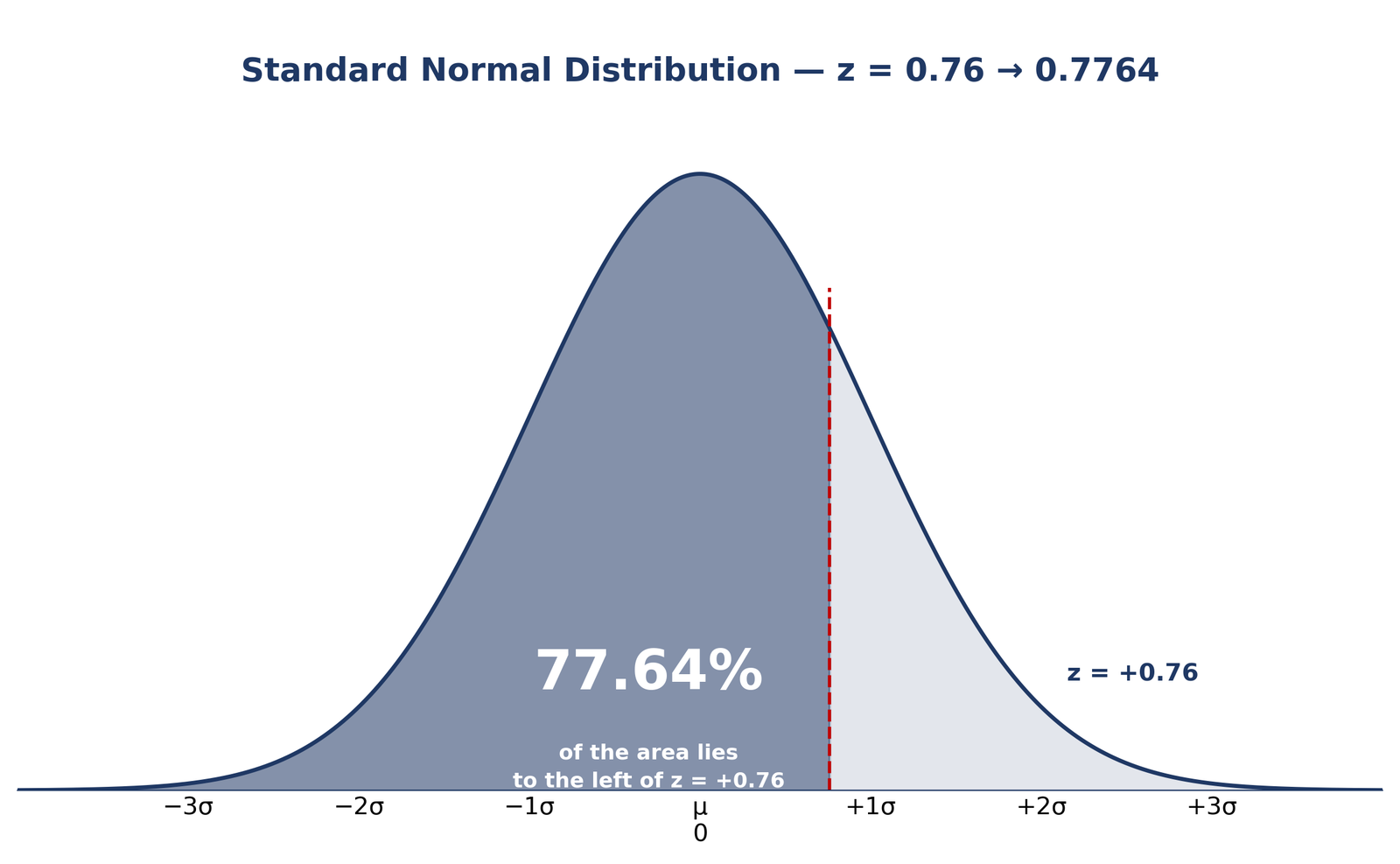
Example 1 — Area to the Left of z = +0.76

Find Φ(0.76), the area to the left of z = +0.76. The table gives Φ(0.76) = 0.7764. So 77.64% of the standard normal distribution lies below z = +0.76, and the remaining 22.36% lies above it.

Example 2 — Left Tail at z = +1.21

Find P(Z < 1.21). This is a left-tail probability, so it is Φ(1.21) directly from the table: Φ(1.21) = 0.8869. About 88.69% of values fall below z = +1.21.

Example 3 — Right Tail Above z = −0.44

Find P(Z > −0.44). The table gives left-tail areas, so use the symmetry of the curve: P(Z > −0.44) = P(Z < +0.44) = Φ(0.44) = 0.6700. About 67.00% of values lie above z = −0.44.

Example 4 — Between z = −0.64 and z = +2.27

Find P(−0.64 < Z < 2.27). Subtract the two left-tail areas: Φ(2.27) − Φ(−0.64) = 0.9884 − 0.2611 = 0.7273. About 72.73% of the distribution lies between these two z-scores.

Example 5 — Reverse Lookup: Probability to Z-Score

Find the z-score with 0.8051 of the area to its left. Look for 0.8051 inside the standard normal table: it sits at z ≈ +0.86, since Φ(0.86) = 0.8051. Reverse lookups like this are how percentiles are turned back into scores — try one yourself with the probability to z-score tool.

Example 6 — IQ Above 140 (Genius Range)

IQ scores are approximately normal with μ = 100 and σ = 15. What proportion of people score above 140? First convert: Z = (140 − 100) / 15 = 40 / 15 = +2.67. Then Φ(2.67) = 0.9962, so the area above is 1 − 0.9962 = 0.0038. Only about 0.38% of people — roughly 4 in 1,000 — score above 140.

Example 7 — IQ of 130 as a Percentile

An IQ of 130 has Z = (130 − 100) / 15 = +2.00. From the table, Φ(2.00) = 0.9772, so an IQ of 130 is at the 97.72nd percentile: higher than about 98 in 100 people. You can convert any z-score to a percentile instantly with the z-score to percentile converter.

Example 8 — Test Score of 85

A test is approximately normal with μ = 70 and σ = 10. A score of 85 has Z = (85 − 70) / 10 = +1.50, and Φ(1.50) = 0.9332, so 85 is at the 93.32nd percentile. To see where a score like this sits on the curve, plot the z-score on a bell curve with the graph plotter.

Finding a probability from the standard normal distribution is a three-step routine: convert to a z-score if you do not already have one, decide which area you need — left tail, right tail or between two values — and read Φ(z) from the table or a calculator.

• Left tail, P(Z < z): read Φ(z) straight from the table.
• Right tail, P(Z > z): use 1 − Φ(z).
• Between two values, P(a < Z < b): use Φ(b) − Φ(a).
• Probability to z-score: find the probability inside the table and read the z-score from the row and column — the reverse of the steps above.

For a worked reminder of the table itself, see how to read a z-table. For exact probabilities without a table, use the Normal Distribution Calculator and compare its answer with the table value.

A standard normal table lists Φ(z) — the area to the left of each z-score — usually for z from −3.49 to +3.49 in steps of 0.01. To use it, split the z-score into a row and a column: the row gives the z-score to one decimal place, and the column gives the second decimal place. For z = +0.76, find row 0.7 and column 0.06; the entry where they meet is 0.7764.

For negative z-scores, use symmetry: Φ(−z) = 1 − Φ(z). So Φ(−0.64) = 1 − Φ(0.64) = 1 − 0.7389 = 0.2611. Some tables list negative z-scores directly; either way, the answer is the same. Remember that a table entry is always a left-tail area, so right-tail and between-values probabilities need the subtractions shown above — never read a right-tail probability straight off the table.

Every standard normal distribution is a normal distribution, but most normal distributions are not standard. The difference is only the centre and the scale.

Feature	Normal distribution	Standard normal distribution
Notation	X ~ N(μ, σ²)	Z ~ N(0, 1)
Mean	μ (any value)	0
Standard deviation	σ (any positive value)	1
Horizontal axis	Original units (points, inches, mmHg)	Z-scores (standard deviations)
Probability table	Would need a new table for every μ and σ	One table works for every case
Shape	Bell-shaped and symmetric	Bell-shaped and symmetric

Short answer: a normal distribution has any mean and standard deviation, while the standard normal distribution is the special case with mean 0 and standard deviation 1. Standardizing — subtracting μ and dividing by σ — turns any normal distribution into the standard one.

Normal Approximation to the Binomial

The standard normal distribution can also approximate a binomial distribution when the sample is large enough. The approximation works when both np > 5 and n(1 − p) > 5, where n is the number of trials and p is the probability of success on each trial. Under those conditions, the binomial count X is approximately normal with mean μ = np and standard deviation σ = √(np(1 − p)).

Because the binomial is discrete and the normal curve is continuous, apply a continuity correction: move the boundary by 0.5 towards the centre of the range you want. For P(X ≤ 22) with n = 50 and p = 0.4, use 22.5 as the boundary. The mean is μ = 50 × 0.4 = 20 and the standard deviation is σ = √(50 × 0.4 × 0.6) = √12 ≈ 3.46, so Z = (22.5 − 20) / 3.46 ≈ +0.72, and Φ(0.72) = 0.7642. The approximation gives about 76.42% — close to the exact binomial probability. If np or n(1 − p) is 5 or less, do not use the approximation; use the exact binomial probabilities instead.

Is the Standard Normal Distribution the Same as a Z-Distribution?

Yes. “Z-distribution” is just a shorter name for the standard normal distribution, the distribution of z-scores, Z ~ N(0, 1). Textbooks and calculators use the two names interchangeably, so a “z-table” and a “standard normal table” are the same table.

What Is the Z-Score in a Standard Normal Distribution?

In the standard normal distribution, the value itself is the z-score. A value of Z = +1.50 means 1.50 standard deviations above the mean, and its percentile is Φ(1.50) × 100 = 93.32. Negative z-scores sit below the mean: Z = −1.00 is one standard deviation below the mean, with Φ(−1.00) = 0.1587, or the 15.87th percentile.

Can a Standard Normal Distribution Have a Negative Z-Score?

Yes. About half of all z-scores are negative, because the curve is centred at 0 and symmetric. A negative z-score simply means the value is below the mean. For example, Z = −0.44 has 33.00% of the area to its left and 67.00% to its right, since Φ(−0.44) = 0.3300.

Standard Normal Distribution Practice Problems

Try these five problems, then check your answers. Use the standard normal table, or check yourself with the Bell Curve Generator to picture each area.

1. Find P(Z < 1.00). Answer: 0.8413
2. Find P(Z > −1.00). Answer: 0.8413
3. Find P(−1 < Z < 1). Answer: 0.6827
4. What z-score marks the 95th percentile? Answer: +1.645
5. Convert X = 115 to a z-score when μ = 100 and σ = 15. Answer: z = +1.00

Notice that problems 1 and 2 have the same answer: by symmetry, the area below +1 equals the area above −1. Problem 3 is the 68.27% interval from the 68-95-99.7 rule, and problem 4 is the z-score used for one-sided 95% confidence limits.

Frequently Asked Questions

What is the standard normal distribution?

The standard normal distribution is the normal distribution with mean 0 and standard deviation 1, written Z ~ N(0, 1). It is the bell-shaped distribution of z-scores, and a single standard normal table gives probabilities for every normal distribution once its values have been standardized.

What are the mean and standard deviation of the standard normal distribution?

The mean is 0 and the standard deviation is 1. Its variance is also 1, its median and mode are both 0, and the total area under its curve is 1.

How do you convert a normal distribution to the standard normal distribution?

Convert each value X to a z-score with Z = (X − μ) / σ: subtract the mean μ from the value, then divide by the standard deviation σ. The resulting z-scores follow the standard normal distribution, Z ~ N(0, 1).

What are some standard normal distribution examples?

Φ(0.76) = 0.7764, so 77.64% of the area lies below z = +0.76; P(Z < 1.21) = 0.8869; P(Z > −0.44) = 0.6700; and P(−0.64 < Z < 2.27) = 0.7273. An IQ of 140 (μ = 100, σ = 15) has z = +2.67, so only 0.38% of people score above it.

How does the standard normal distribution differ from a normal distribution?

A normal distribution can have any mean μ and standard deviation σ, while the standard normal distribution is the special case with μ = 0 and σ = 1. Standardizing any normal distribution — subtracting μ and dividing by σ — turns it into the standard normal distribution.

How do you find probability using the standard normal distribution?

Convert the value to a z-score with Z = (X − μ) / σ, then read Φ(z) from the standard normal table. For a left tail, use Φ(z); for a right tail, use 1 − Φ(z); for the area between two values, use Φ(b) − Φ(a).

How do you use a standard normal distribution table?

Find the z-score’s first decimal in the row and its second decimal in the column; the entry where they meet is Φ(z), the area to the left of z. For example, row 0.7 and column 0.06 give Φ(0.76) = 0.7764. For negative z, use Φ(−z) = 1 − Φ(z).

Where can I find standard normal distribution practice problems?

On this page: P(Z < 1.00) = 0.8413, P(Z > −1.00) = 0.8413, P(−1 < Z < 1) = 0.6827, the 95th percentile is z = +1.645, and X = 115 (μ = 100, σ = 15) converts to z = +1.00.

For the theory behind the curve, see the NIST/SEMATECH e-Handbook of Statistical Methods.

Check Tools

Put the standard normal distribution into practice with these free tools.