Learning how to read a z table is one of the fastest skills in statistics: once you can read one row and one column, you can turn any z-score into a probability in seconds. A z-table — also called a standard normal table, a z-score table, or a normal distribution table — lists the area under the standard normal curve for z-scores from 0.00 to 3.49. This guide shows you the three table layouts, the exact lookup steps for left-tail, right-tail, and between-values problems, negative z-scores, and reverse lookup, with worked examples you can check against the full printable table at the end.
If you do not have a z-score yet, learn how to calculate a z-score in our companion guide first, or use the z-score calculator to get one. Then come back here to look it up.
What Is a Z-Table?
A z-table is a printed table of the standard normal distribution — the bell curve with mean 0 and standard deviation 1. For each z-score, the table gives the area under that curve, which is a probability. Because the total area under the curve is 1, every area the table gives is a number between 0 and 1, and it can always be read as a percentage.
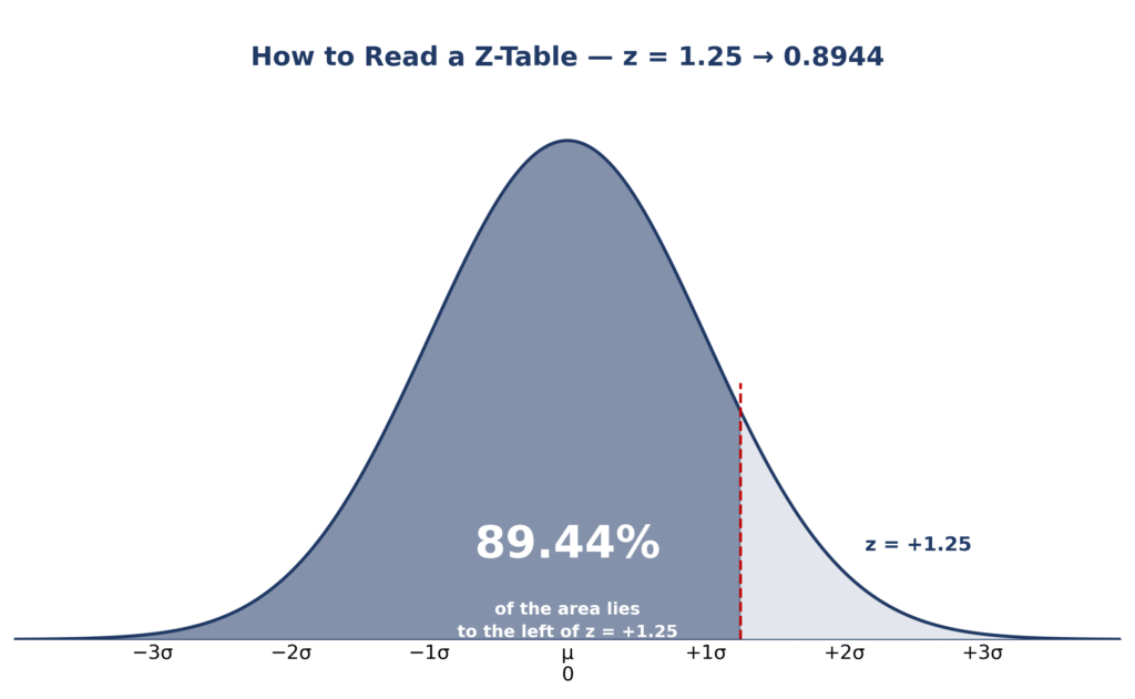
For example, the table says the area to the left of z = 1.25 is 0.8944. That means 89.44% of values in a standard normal distribution fall below a z-score of 1.25. The same idea works for test scores, heights, IQ scores, and any data that is approximately normal: convert a raw score to a z-score, then read the probability from the z-table.
A z-table chart usually prints z-scores in rows and columns. The row gives the z-score to one decimal place (0.0, 0.1, 0.2, and so on), and the column gives the second decimal place (0.00 to 0.09). The cell where a row and a column meet is the probability. That row-and-column structure is the whole trick — and the most common source of mistakes, as the common mistakes section below shows.
The 3 Z-Table Layouts (and How to Convert Between Them)
Not all z-tables print the same area. Before you read a value, check which layout your table uses — a 0.8413 in one layout is a 0.3413 in another. The three layouts are:
- Cumulative table (most common): gives the area to the left of z, written Φ(z). For z = 1.00, it reads 0.8413.
- Mean-to-z table: gives the area between the mean (z = 0) and z. For z = 1.00, it reads 0.3413.
- Right-tail table: gives the area to the right of z. For z = 1.00, it reads 0.1587.
All three describe the same curve, so you can convert between them with simple arithmetic:
| If your table gives | Left area Φ(z) | Mean-to-z area | Right-tail area |
|---|---|---|---|
| Left area Φ(z) = A | A | A − 0.5000 | 1 − A |
| Mean-to-z area = B | 0.5000 + B | B | 0.5000 − B |
| Right-tail area = C | 1 − C | 0.5000 − C | C |
Check it with z = 1.00: the cumulative table says 0.8413, so the mean-to-z area is 0.8413 − 0.5000 = 0.3413, and the right tail is 1 − 0.8413 = 0.1587. The printable table at the end of this page is a cumulative table, and every worked example below uses that layout unless it says otherwise.
How to Use a Z-Table
Follow these four steps for every lookup:
- Get your z-score. If you have a raw score x from a normal distribution with mean μ and standard deviation σ, convert it with z = (x − μ) / σ. Our free z-score tool does this for you.
- Split the z-score into a row and a column. The row is the z-score to one decimal place; the column is the second decimal place. For z = 1.25, the row is 1.2 and the column is 0.05.
- Find the row and column in the table. Run your finger along the 1.2 row until you reach the 0.05 column. The number in that cell is your answer.
- Read the value and name the area. In a cumulative table, the cell is the area to the left of z — the probability that a value is below your z-score. For z = 1.25, the cell reads 0.8944, so 89.44% of the distribution lies below it.
That is all there is to it. The rest of this guide applies those four steps to each kind of question a z-table can answer.
How to Read a Z-Table for Left Tail
The left tail is the area to the left of a z-score — the most common question, because a cumulative z-table gives it directly. Worked example with z = 1.25:
- Split z = 1.25. Row 1.2, column 0.05.
- Find the cell. In the 1.2 row, under the 0.05 column, the table reads 0.8944.
- Read the answer. The area to the left of z = 1.25 is 0.8944, so P(Z < 1.25) = 0.8944, or 89.44%.
Two more left-tail lookups using the same steps:
- z = 1.00: row 1.0, column 0.00 → 0.8413. So 84.13% of the distribution lies below z = 1.00.
- z = 1.09: row 1.0, column 0.09 → 0.8621. So P(Z < 1.09) = 0.8621, or 86.21%.
Check any left-tail answer instantly with our z-score to percentile converter — enter the z-score and it returns the same percentile the table gives.
Z-Table Negative Z-Score
Many printed tables only list positive z-scores. For a negative z-score, use the symmetry of the bell curve: the area to the left of −z equals the area to the right of +z, so Φ(−z) = 1 − Φ(z).
Worked example, z = −1.25: the table gives Φ(1.25) = 0.8944, so Φ(−1.25) = 1 − 0.8944 = 0.1056. Only 10.56% of the distribution lies below z = −1.25.
The same rule works in reverse: the area to the right of a negative z-score equals the area to the left of its positive twin. For example, the area to the right of z = −1.00 is 0.8413, because the area to the left of z = +1.00 is 0.8413.
Never read a negative z-score from the positive side of the table without subtracting from 1 — that is the single most common z-table error.
How to Find Probability from Z-Table
A cumulative z-table gives the left tail directly. Every other probability is one subtraction away:
- Left tail, P(Z < z): read the cell. P(Z < 1.25) = 0.8944.
- Right tail, P(Z > z): 1 − the cell. P(Z > 1.25) = 1 − 0.8944 = 0.1056.
- Between two values, P(a < Z < b): Φ(b) − Φ(a). See the next section.
- Outside two values: 1 − the between area.
Worked example — a hypothesis test with z = 2.25. The table gives Φ(2.25) = 0.9878, so the right-tail probability is 1 − 0.9878 = 0.0122. That is the one-tailed p-value. For a two-tailed test, double it: p = 2 × 0.0122 = 0.0244. If you want to skip the table, our p-value calculator from z-score gives the same result, and the left/right tail probability calculator checks any left- or right-tail area.
Z-Table Between Two Values
To find the probability between two z-scores, look up both and subtract the smaller area from the larger one: P(a < Z < b) = Φ(b) − Φ(a).
Worked example — between z = −1 and z = +1: Φ(1.00) = 0.8413 and Φ(−1.00) = 1 − 0.8413 = 0.1587, so P(−1 < Z < 1) = 0.8413 − 0.1587 = 0.6827. That is the familiar 68.27% from the empirical rule — about 68% of values fall within one standard deviation of the mean.
Worked example — between z = 1.00 and z = 1.25: Φ(1.25) − Φ(1.00) = 0.8944 − 0.8413 = 0.0531, so 5.31% of values fall between those two z-scores.
Always subtract in the right order: the larger z-score’s area minus the smaller z-score’s area. Subtracting the other way gives a negative probability, which is impossible — a quick sign check that catches the error.
Reverse Z-Table Lookup
Reverse lookup works backwards: you know the probability and need the z-score. Instead of matching a row and column to a cell, scan the body of the table for the probability closest to your target, then read off its row and column.
| Target probability | Nearest table value | z-score |
|---|---|---|
| 0.90 (left tail) | 0.8997 | +1.28 |
| 0.975 (left tail) | 0.9750 | +1.96 |
| 0.05 (left tail) | 0.0500 (as 1 − 0.9500) | −1.645 |
Worked examples: for a 90th percentile, look for 0.9000 in the table; the closest value is 0.8997 at row 1.2, column 0.08, so z ≈ +1.28. For the middle 95% of a normal distribution, the upper cut-off is the 97.5th percentile: the table shows 0.9750 at z = +1.96. For a 5% left tail, find 0.9500 (z = +1.645) and flip the sign: z = −1.645.
These are the critical values used everywhere in statistics: ±1.645 for 90% confidence, ±1.96 for 95% confidence, and ±2.58 for 99% confidence (the table gives Φ(2.58) = 0.9951, the 99.5th percentile). For exact values without scanning the table, use our probability to z-score tool.
Z-Table vs Z-Score Calculator
A z-table and a z-score calculator answer different halves of the same question. A z-score calculator turns a raw score into a z-score; a z-table turns a z-score into a probability. Use the table when you are learning, when you are in an exam without a calculator, or when you want to see how probabilities change as z grows. Use a calculator when you need more than four decimals, when your z-score has more than two decimal places, or when you are checking a table answer. The z-score graph plotter shows the same area on the curve, which makes the table’s numbers visual. Both routes should agree: if the table says 0.8944 for z = 1.25, the calculator should say the same.
Common Mistakes When Reading a Z-Table
- Reading the wrong layout. Check whether your table gives the left area, the mean-to-z area, or the right tail before you read a single value. A mean-to-z table says 0.3413 where a cumulative table says 0.8413 for the same z = 1.00.
- Mixing up the row and column. For z = 1.25, the row is 1.2 and the column is 0.05 — not row 1.5, column 0.02. The first decimal is the row; only the second decimal is the column.
- Forgetting the negative sign. A negative z-score needs Φ(−z) = 1 − Φ(z). Reading Φ(1.25) = 0.8944 for z = −1.25 gives 0.8944 instead of the correct 0.1056.
- Subtracting the wrong way round. Between two values, always subtract the smaller area from the larger one. A negative probability means the subtraction is backwards.
- Reading a probability as a z-score. In reverse lookup, scan the body of the table for the probability, then read the row and column. The number in the body is never the z-score.
- Rounding too early. Keep four decimals through your working and round only the final answer.
Why Do Z-Tables Only Go Up to 3.49?
Because beyond z = 3.49, the cumulative probability is 0.9998 or more — the area is so close to 1 that four-decimal tables cannot show any further change. The chance of a value beyond z = 3.49 is less than 0.02%, so tables stop there and calculators take over for extreme values.
What Is the Difference Between a Z-Table and a Normal Distribution Table?
There is none — a normal distribution table is another name for a z-table. Both list areas under the standard normal curve. The only real difference is the layout: some tables print the cumulative (left-tail) area, others print the mean-to-z area or the right tail. Check the layout first, using the conversion table above, and any of them will give the same answer.
Can a Z-Table Give a P-Value?
Yes. A p-value is a tail probability, and a z-table gives tail probabilities. For a one-tailed test, the p-value is the area beyond your z-score: for z = 2.25, p = 1 − 0.9878 = 0.0122. For a two-tailed test, double it: p = 0.0244. If that p-value is below your significance level (usually 0.05), the result is statistically significant.
Z-Table 0.00 to 3.49 Printable
Below is the full cumulative z-table: the area to the left of each z-score, Φ(z), to four decimals. Find your z-score’s row (first decimal) and column (second decimal). For negative z-scores, use Φ(−z) = 1 − Φ(z). Nine anchor values to check: z = 0.00 → 0.5000, z = 0.50 → 0.6915, z = 1.00 → 0.8413, z = 1.25 → 0.8944, z = 1.96 → 0.9750, z = 2.00 → 0.9772, z = 2.58 → 0.9951, z = 3.00 → 0.9987, and z = 3.49 → 0.9998.
| z | 0.00 | 0.01 | 0.02 | 0.03 | 0.04 | 0.05 | 0.06 | 0.07 | 0.08 | 0.09 |
|---|---|---|---|---|---|---|---|---|---|---|
| 0.0 | 0.5000 | 0.5040 | 0.5080 | 0.5120 | 0.5160 | 0.5199 | 0.5239 | 0.5279 | 0.5319 | 0.5359 |
| 0.1 | 0.5398 | 0.5438 | 0.5478 | 0.5517 | 0.5557 | 0.5596 | 0.5636 | 0.5675 | 0.5714 | 0.5753 |
| 0.2 | 0.5793 | 0.5832 | 0.5871 | 0.5910 | 0.5948 | 0.5987 | 0.6026 | 0.6064 | 0.6103 | 0.6141 |
| 0.3 | 0.6179 | 0.6217 | 0.6255 | 0.6293 | 0.6331 | 0.6368 | 0.6406 | 0.6443 | 0.6480 | 0.6517 |
| 0.4 | 0.6554 | 0.6591 | 0.6628 | 0.6664 | 0.6700 | 0.6736 | 0.6772 | 0.6808 | 0.6844 | 0.6879 |
| 0.5 | 0.6915 | 0.6950 | 0.6985 | 0.7019 | 0.7054 | 0.7088 | 0.7123 | 0.7157 | 0.7190 | 0.7224 |
| 0.6 | 0.7257 | 0.7291 | 0.7324 | 0.7357 | 0.7389 | 0.7422 | 0.7454 | 0.7486 | 0.7517 | 0.7549 |
| 0.7 | 0.7580 | 0.7611 | 0.7642 | 0.7673 | 0.7704 | 0.7734 | 0.7764 | 0.7794 | 0.7823 | 0.7852 |
| 0.8 | 0.7881 | 0.7910 | 0.7939 | 0.7967 | 0.7995 | 0.8023 | 0.8051 | 0.8078 | 0.8106 | 0.8133 |
| 0.9 | 0.8159 | 0.8186 | 0.8212 | 0.8238 | 0.8264 | 0.8289 | 0.8315 | 0.8340 | 0.8365 | 0.8389 |
| 1.0 | 0.8413 | 0.8438 | 0.8461 | 0.8485 | 0.8508 | 0.8531 | 0.8554 | 0.8577 | 0.8599 | 0.8621 |
| 1.1 | 0.8643 | 0.8665 | 0.8686 | 0.8708 | 0.8729 | 0.8749 | 0.8770 | 0.8790 | 0.8810 | 0.8830 |
| 1.2 | 0.8849 | 0.8869 | 0.8888 | 0.8907 | 0.8925 | 0.8944 | 0.8962 | 0.8980 | 0.8997 | 0.9015 |
| 1.3 | 0.9032 | 0.9049 | 0.9066 | 0.9082 | 0.9099 | 0.9115 | 0.9131 | 0.9147 | 0.9162 | 0.9177 |
| 1.4 | 0.9192 | 0.9207 | 0.9222 | 0.9236 | 0.9251 | 0.9265 | 0.9279 | 0.9292 | 0.9306 | 0.9319 |
| 1.5 | 0.9332 | 0.9345 | 0.9357 | 0.9370 | 0.9382 | 0.9394 | 0.9406 | 0.9418 | 0.9429 | 0.9441 |
| 1.6 | 0.9452 | 0.9463 | 0.9474 | 0.9484 | 0.9495 | 0.9505 | 0.9515 | 0.9525 | 0.9535 | 0.9545 |
| 1.7 | 0.9554 | 0.9564 | 0.9573 | 0.9582 | 0.9591 | 0.9599 | 0.9608 | 0.9616 | 0.9625 | 0.9633 |
| 1.8 | 0.9641 | 0.9649 | 0.9656 | 0.9664 | 0.9671 | 0.9678 | 0.9686 | 0.9693 | 0.9699 | 0.9706 |
| 1.9 | 0.9713 | 0.9719 | 0.9726 | 0.9732 | 0.9738 | 0.9744 | 0.9750 | 0.9756 | 0.9761 | 0.9767 |
| 2.0 | 0.9772 | 0.9778 | 0.9783 | 0.9788 | 0.9793 | 0.9798 | 0.9803 | 0.9808 | 0.9812 | 0.9817 |
| 2.1 | 0.9821 | 0.9826 | 0.9830 | 0.9834 | 0.9838 | 0.9842 | 0.9846 | 0.9850 | 0.9854 | 0.9857 |
| 2.2 | 0.9861 | 0.9864 | 0.9868 | 0.9871 | 0.9875 | 0.9878 | 0.9881 | 0.9884 | 0.9887 | 0.9890 |
| 2.3 | 0.9893 | 0.9896 | 0.9898 | 0.9901 | 0.9904 | 0.9906 | 0.9909 | 0.9911 | 0.9913 | 0.9916 |
| 2.4 | 0.9918 | 0.9920 | 0.9922 | 0.9925 | 0.9927 | 0.9929 | 0.9931 | 0.9932 | 0.9934 | 0.9936 |
| 2.5 | 0.9938 | 0.9940 | 0.9941 | 0.9943 | 0.9945 | 0.9946 | 0.9948 | 0.9949 | 0.9951 | 0.9952 |
| 2.6 | 0.9953 | 0.9955 | 0.9956 | 0.9957 | 0.9959 | 0.9960 | 0.9961 | 0.9962 | 0.9963 | 0.9964 |
| 2.7 | 0.9965 | 0.9966 | 0.9967 | 0.9968 | 0.9969 | 0.9970 | 0.9971 | 0.9972 | 0.9973 | 0.9974 |
| 2.8 | 0.9974 | 0.9975 | 0.9976 | 0.9977 | 0.9977 | 0.9978 | 0.9979 | 0.9979 | 0.9980 | 0.9981 |
| 2.9 | 0.9981 | 0.9982 | 0.9982 | 0.9983 | 0.9984 | 0.9984 | 0.9985 | 0.9985 | 0.9986 | 0.9986 |
| 3.0 | 0.9987 | 0.9987 | 0.9987 | 0.9988 | 0.9988 | 0.9989 | 0.9989 | 0.9989 | 0.9990 | 0.9990 |
| 3.1 | 0.9990 | 0.9991 | 0.9991 | 0.9991 | 0.9992 | 0.9992 | 0.9992 | 0.9992 | 0.9993 | 0.9993 |
| 3.2 | 0.9993 | 0.9993 | 0.9994 | 0.9994 | 0.9994 | 0.9994 | 0.9994 | 0.9995 | 0.9995 | 0.9995 |
| 3.3 | 0.9995 | 0.9995 | 0.9995 | 0.9996 | 0.9996 | 0.9996 | 0.9996 | 0.9996 | 0.9996 | 0.9997 |
| 3.4 | 0.9997 | 0.9997 | 0.9997 | 0.9997 | 0.9997 | 0.9997 | 0.9997 | 0.9997 | 0.9997 | 0.9998 |
Tip: to check any value in this table, enter the z-score in our z-score to percentile tool — it should match the table to four decimals.
Frequently Asked Questions
How do you read a z-table step by step?
Split the z-score into a row (first decimal) and a column (second decimal), then read the cell where they meet. For z = 1.25, row 1.2 and column 0.05 give 0.8944 — the area to the left of z = 1.25.
What does 0.8413 mean in a z-table?
It is the area to the left of z = 1.00: 84.13% of values in a standard normal distribution fall below a z-score of 1.00. The same z-score gives a mean-to-z area of 0.3413 and a right-tail area of 0.1587.
How do you read a z-table for a negative z-score?
Use symmetry: Φ(−z) = 1 − Φ(z). Look up the positive z-score and subtract from 1. For z = −1.25, Φ(−1.25) = 1 − 0.8944 = 0.1056.
How do you find the probability between two z-scores?
Look up both values and subtract the smaller area from the larger one: P(a < Z < b) = Φ(b) − Φ(a). Between z = −1 and z = +1, that is 0.8413 − 0.1587 = 0.6827.
How do you do a reverse z-table lookup?
Find the probability inside the body of the table and read its row and column as the z-score. The closest value to 0.9000 is 0.8997, at row 1.2 and column 0.08, so z ≈ +1.28. A probability of 0.9750 gives z = +1.96.
What is the z-score for the 95th percentile?
About +1.645. The table shows 0.9495 at z = 1.64 and 0.9505 at z = 1.65, so the 95th percentile sits between them, at z ≈ 1.645.
Is a z-table the same as a standard normal table?
Yes. “Standard normal table”, “z-score table”, “z-table chart”, and “normal distribution table” are all names for the same table. Only the layout can differ — cumulative, mean-to-z, or right-tail — so check which area your table prints before you read it.
When should I use a z-table instead of a calculator?
Use the table when you are learning, revising, or in an exam where only a printed table is allowed. Use a calculator when your z-score has more than two decimal places, when you need more than four decimals of precision, or when you want to check a table answer.
Conclusion
Reading a z-table comes down to three things: know your table’s layout, split the z-score into a row and a column, and name the area you just read. With those steps, z = 1.25 always gives 0.8944, a negative z-score is one subtraction away, and a probability between two values is a subtraction of two lookups. Keep the printable table above handy, and check every answer with the percentile converter or the probability to z-score converter until the steps feel automatic.
Reference: the standard normal distribution and its tables are documented in the NIST/SEMATECH e-Handbook of Statistical Methods.
Check Tools
Try these free tools to check your z-table answer or skip the table altogether:
Z-Score Calculator
Turn any value into a z-score, percentile and probability.
ToolsTry Calculator → ● LiveZ-Score Graph Plotter
Plot a z-score on a bell curve and shade the area it cuts off.
ToolsTry Calculator → ● LiveZ-Score to Percentile Converter
Convert any z-score into its exact percentile in one step.
ToolsTry Calculator → ● LiveProbability to Z-Score Approximation Tool
Work backwards from a probability to the z-score that produces it.
ToolsTry Calculator → ● LiveLeft/Right Tail Probability Calculator
Find the area in either tail for any z-score, without the table.
ToolsTry Calculator → ● LiveEmpirical Rule Percentile Calculator
Convert percentiles to values with a mean and SD.
ToolsTry Calculator → ● LiveExplore All Statistical Tools
Browse every free calculator on this site.
ToolsTry Calculator →Check Articles
How to Calculate a Z-Score
A z-score tells you how many standard deviations a value sits from the mean.
ArticleRead Article → ● LiveWhat is the Empirical Rule?
The 68.27%, 95.45% and 99.73% shares explained from the start.
ArticleRead Article → ● LiveNormal Distribution and the Empirical Rule
How the bell curve works, and why it makes the rule possible.
ArticleRead Article → ● LiveHow to Use Empirical Rule Calculator
Worked steps for the calculator, from mean and standard deviation to results.
ArticleRead Article → ● LiveReal-Life Applications of Percentiles in Normal Distribution
Real-life applications of percentiles in normal distribution turn a score into a rank.
ArticleRead Article → ● LiveEmpirical Rule vs. Confidence Intervals: What’s the Difference?
The empirical rule and the confidence interval are not the same thing.
ArticleRead Article →