
What Is a Bell Curve?
If you have ever been graded on a curve, taken an IQ test or read that a result was “within the normal range”, you have already met a bell curve. It is the shape that appears whenever many small, unrelated influences add up — and once you can read it, a single picture tells you how common or rare any value is.
A bell curve is the graph of a normal distribution: a smooth, symmetric curve with a single peak at the mean. The curve never touches the horizontal axis, and its spread is fixed by the standard deviation.
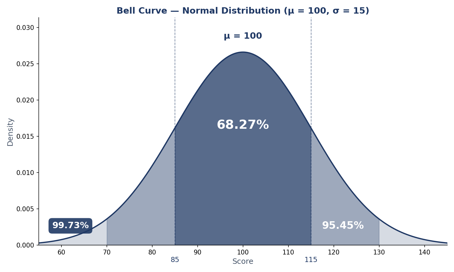
A bell curve is the graph of a normal distribution: a smooth, symmetric curve with most values clustered around the mean and fewer in the tails. About 68.27% of values fall within one standard deviation of the mean, 95.45% within two and 99.73% within three.
What Is a Bell Curve?
A bell curve is the graph of a normal distribution: a smooth, symmetric curve with a single peak at the mean and tails that fall away evenly on both sides. Most values cluster near the centre and very few sit far away. That is why the normal distribution is the most used distribution in statistics — it describes IQ scores, heights, test marks and measurement errors.
Mathematicians write a normal distribution as X ~ N(μ, σ²), where μ (mu) is the mean and σ (sigma) is the standard deviation. The curve itself is the probability density function:
f(x) = 1 / (σ√(2π)) × e−(x−μ)² / (2σ²)
You do not need to memorise the formula to use a bell curve. What matters is what the two parameters do: the mean sets where the peak sits, and the standard deviation sets how wide the curve is. Change the mean and the curve slides left or right; change the standard deviation and it stretches or squeezes. To see that, open our bell curve generator, set a mean and a standard deviation, and watch the curve move.
A bell curve has four properties worth remembering. It is symmetric: the left half mirrors the right. It is unimodal: it has exactly one peak, where the mean, median and mode all sit. Its tails are asymptotic: the curve approaches the horizontal axis but never touches it, so extreme values are possible but very unlikely. And the total area under the curve is exactly 1, so areas under it are probabilities. The classic normal distribution examples on this site — heights, IQ scores and test marks — show all four in action.
Why Is It Called a Bell Curve?
Because of its shape. Plot the heights of a large group of adults and the outline rises gently, peaks in the middle and falls away to the right — the silhouette of a hand bell. The mathematics is older than the name: Abraham de Moivre described the curve in 1733, Carl Friedrich Gauss used it in 1809 for the theory of errors (hence “Gaussian distribution”), and by the twentieth century “bell curve” had become its everyday name.
The 68-95-99.7 Rule, Exactly
You have probably seen the rule written as 68-95-99.7: about 68% of values within one standard deviation of the mean, 95% within two, 99.7% within three. Those are rounded figures. The exact percentages, for a truly normal distribution, are 68.27%, 95.45% and 99.73%. The rounded versions are fine for quick talk; the exact versions are what you should use when you calculate. The rule itself is the empirical rule, and it is the single most useful fact about a bell curve.
It helps to split each band into its two sides. Because the curve is symmetric, each side holds exactly half of the band. The empirical rule graph generator draws these bands for any mean and standard deviation you enter:
| Band (one side) | Share of values |
|---|---|
| Mean to 1σ | 34.13% |
| 1σ to 2σ | 13.59% |
| 2σ to 3σ | 2.14% |
| Beyond 3σ | 0.13% |
Read the table from the centre outwards. A value between the mean and one standard deviation above it is common — 34.13% of all values sit in that slice. Between one and two standard deviations, 13.59%. Between two and three, 2.14%. Beyond three, just 0.13% — about one value in 750. The same figures apply on the low side, by symmetry.
The steps between the headline numbers matter too. Going from one standard deviation to two adds 95.45 − 68.27 = 27.18% — the two 13.59% slices. Going from two to three adds 99.73 − 95.45 = 4.28% — the two 2.14% slices. The curve’s bulk sits in the middle.
If you want the picture rather than the table, see all three bands on one curve with your own numbers. The U.S. National Institute of Standards and Technology describes the normal distribution and its percentages in its Engineering Statistics Handbook (1.3.6.6.1. Normal Distribution).
How to Read a Bell Curve
Reading a bell curve means turning a value into two numbers: a z-score and a percentile. The z-score says how many standard deviations the value sits from the mean: z = (x − μ) / σ. The percentile says what share of values fall below it. Our guide to how to calculate a z-score walks through the conversion, and how to read a z-table shows the lookup step.
Take IQ scores, the classic bell curve, with a mean of 100 and a standard deviation of 15. The bands are: 68.27% of people score between 85 and 115, 95.45% between 70 and 130, and 99.73% between 55 and 145. A score of 130 is z = (130 − 100) / 15 = +2.00, the 97.72nd percentile — only 2.28% of people score above it. A score of 115 is z = +1.00, the 84.13th percentile. And the 90th percentile, the score that beats 90% of people, is 119.22.
The same reading works for any bell-shaped data. On a class test with a mean of 72 and a standard deviation of 6, 68.27% scored between 66 and 78 and 95.45% between 60 and 84. A mark of 84 is two standard deviations above the mean — the 97.72nd percentile.
Try it in the generator: draw your own curve with any mean and standard deviation, then plot a z-score on the curve and read off the percentile.
Bell Curve vs Histogram
A histogram and a bell curve look alike at a glance, but they are different objects. A histogram is a bar chart of real data: each bar’s height is a count of the values in that bin. A bell curve is a smooth density: its height at any point is a probability density, not a probability — the probability of a range is the area under the curve over that range, not the height.
That distinction matters. The peak of a bell curve is the tallest point on the graph, but it is not “the most likely value” as a probability: for a continuous variable, the chance of any exact value is zero. What the peak says is that values near the mean are the densest. A histogram’s tallest bar, by contrast, really does hold the most values.
What Is the Standard Normal Bell Curve?
The standard normal distribution is the bell curve with mean 0 and standard deviation 1, written Z ~ N(0, 1). It is the reference curve for all the others: any normal value converts to it with z = (x − μ) / σ, which is why a single z-table serves every normal distribution. On it, the 68.27% band is z = −1 to +1, the 95.45% band is −2 to +2, and the 99.73% band is −3 to +3. The normal distribution and the empirical rule guide draws exactly this picture, and the z-score graph plotter shades any z-score on it.
How the Mean and Standard Deviation Change the Curve
The mean and the standard deviation are the curve’s only two controls, and each does one job. The mean moves the peak: an IQ curve (μ = 100, σ = 15) and a test-score curve (μ = 70, σ = 15) have the same shape, but one is centred at 100 and the other at 70. The standard deviation sets the width: with the same mean of 100, a σ of 5 gives a tall, narrow bell and a σ of 25 a short, wide one. The total area stays 1 — a wider curve is always a shorter one.
Is Every Dataset Bell-Shaped?
No — and assuming it is will get you into trouble. Income is the classic counterexample: most people earn near the middle, but a long right tail of very high earners pulls the mean above the median, so the distribution is skewed, not symmetric. Other datasets are bimodal (two peaks), flat (uniform, such as a fair die) or heavy-tailed (a few extreme values far from the rest).
The bell curve is a model, not a law of nature. Before you apply the 68-95-99.7 percentages, check the shape with a histogram: if the data is roughly symmetric with one peak and thin tails, the normal model fits. If it is clearly skewed or has two peaks, use a method that does not assume normality — Chebyshev’s theorem guarantees a minimum percentage inside any number of standard deviations for a dataset of any shape.
Frequently Asked Questions
What does a bell curve show?
It shows how values are distributed: how many fall near the mean and how many fall far away. The height at any point is a density, and the area over a range is the share of values in that range.
What is the difference between a bell curve and a normal distribution?
Nothing, in everyday use — a bell curve is the graph of a normal distribution. Strictly, the normal distribution is the mathematical model (defined by its mean and standard deviation) and the bell curve is its picture.
Why is it called a bell curve?
Because the graph looks like a hand bell: it rises gently, peaks in the middle and falls away symmetrically on both sides. The name describes the shape, not the mathematics.
What do the 68-95-99.7 percentages mean, exactly?
They are rounded versions of the exact figures 68.27%, 95.45% and 99.73% — the shares of a normal distribution within one, two and three standard deviations of the mean. Use the exact figures when you calculate.
Is every dataset bell-shaped?
No. Many real datasets are skewed (income), bimodal (two peaks) or flat (uniform). A bell curve is a model that fits some data well and other data badly — always check the shape first.
What is the standard normal distribution?
The normal distribution with mean 0 and standard deviation 1, written Z ~ N(0, 1). Every normal value converts to it with z = (x − μ) / σ, so one z-table serves all normal distributions.
How do the mean and standard deviation change the curve?
The mean moves the peak left or right without changing the shape. The standard deviation widens or narrows the curve: a larger σ makes it shorter and wider, a smaller σ makes it taller and narrower. The area under it stays 1.
Can a bell curve be skewed?
A true bell curve cannot be skewed — symmetry is part of the definition of a normal distribution. If your data is skewed, it is not normal, and you should use a method that does not assume normality, such as Chebyshev’s theorem.
Check Tools
Try the numbers from this guide with the site’s free calculators:
Bell Curve Generator
Draw your own bell curve with any mean and standard deviation, and shade the 68.27%, 95.45% and 99.73% bands.
Try the Bell Curve Generator →
Empirical Rule Graph Generator
See all three bands on one curve.
Try the Empirical Rule Graph Generator →
Z-Score Graph Plotter
Plot any z-score on the curve and read off the area and percentile.
Try the Z-Score Graph Plotter →
Explore All Statistical Tools
Browse every free calculator on the site.
Browse all our statistical tools →
Check Articles
Keep reading with these guides from the site:
What Is the Empirical Rule
The 68-95-99.7 rule in full, with the exact percentages.
Read What Is the Empirical Rule →
Normal Distribution Examples
Heights, IQ scores and test marks, worked through step by step.
Read Normal Distribution Examples →
How to Calculate a Z-Score
Turn any value into a z-score with the (x − μ) / σ formula.
Read How to Calculate a Z-Score →
How to Read a Z-Table
Look up any z-score and read off the area and percentile.
Read How to Read a Z-Table →