
Linear Regression Explained
Linear regression turns a scatter of points into a straight line you can use to predict one variable from another — and, just as importantly, tells you how much to trust that prediction.
Linear regression is the workhorse of statistics: give it pairs of numbers — hours studied and exam scores, advertising spend and sales, temperature and ice-cream sales — and it finds the straight line that fits them best. That line lets you predict new values, and the numbers around it (R², the residuals, the standard error of the slope) tell you whether the line is worth using. This guide works the whole thing out by hand on one real dataset, so you can see every number the calculator produces — and know exactly when not to trust it.
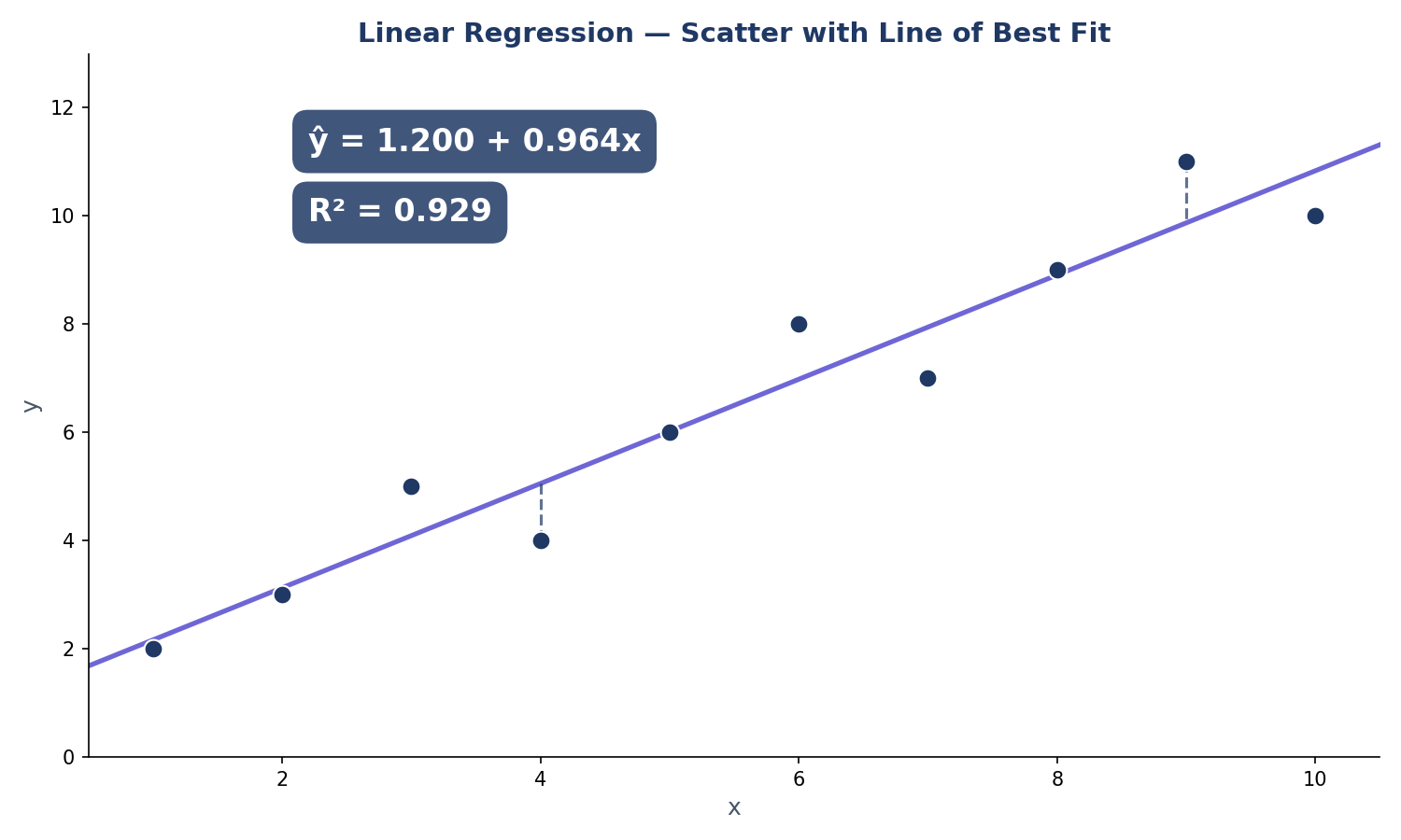
Linear regression fits the straight line that best predicts one variable from another by least squares: it minimises the sum of the squared vertical distances from the points to the line. The line is ŷ = a + bx, where b is the slope and a the intercept.
What Is Linear Regression?
Linear regression is a way to describe the relationship between two variables with a straight line. One variable (x, the predictor) is used to predict the other (y, the response). If the points on a scatter plot roughly follow a straight line, regression gives you that line’s equation — and a set of numbers that say how good the line is.
Think of hours studied (x) against exam score (y), advertising spend (x) against sales (y), or temperature (x) against ice-cream sales (y). In each case the question is the same: if I know x, what y should I expect? You can check every number in this guide with the site’s linear regression calculator — it runs the same ten-point dataset used below.
The line is written ŷ = a + bx. The ŷ (pronounced “y-hat”) is the predicted value of y. The slope b says how much ŷ changes when x increases by 1. The intercept a is the predicted y when x = 0. Note the hat: ŷ is the prediction, y is the actual value, and the difference between them is the residual — the gap the rest of this guide is built on.
This guide covers simple linear regression: one predictor, one response, one straight line. Multiple regression (several predictors at once) uses the same least-squares idea with more terms, but the reading of slope, intercept and R² is the same.
The Least Squares Method
Why this line and not another? The least squares method chooses the line that minimises the sum of the squared vertical distances from the points to the line. For each point, the vertical distance is the residual (y − ŷ). Square each residual, add them up, and you get the sum of squared errors (SSE). The least-squares line is the one with the smallest SSE. Squaring stops positive and negative residuals from cancelling out, and it punishes large misses more than small ones.
The formulas are simple once you have three sums. With x̄ and ȳ the two means, define Sxx = Σ(x − x̄)², Syy = Σ(y − ȳ)² and Sxy = Σ(x − x̄)(y − ȳ). Then the slope is b = Sxy ÷ Sxx and the intercept is a = ȳ − b × x̄. The NIST/SEMATECH e-Handbook of Statistical Methods states the method in exactly these terms, and Newcastle University’s Academic Skills Kit works through the same least-squares formulas with its own worked examples.
The least-squares line always passes through (x̄, ȳ). Whatever your data, the fitted line goes through the point of the two means — a quick check that your hand calculation is on track.
A note on the name: “least squares” is the criterion, not a brand. Any line can be drawn through a scatter of points; least squares picks the one that is closest to all the points at once, in the squared-distance sense.
Fit a Line by Hand in 5 Steps
Here is the whole procedure in five steps. The worked example that follows applies them to one dataset, so you can check each step against real numbers.
- Collect the pairs: write down your x and y values in two columns, one pair per row. Our example uses ten pairs: x = 1, 2, 3, 4, 5, 6, 7, 8, 9, 10 and y = 2, 3, 5, 4, 6, 8, 7, 9, 11, 10.
- Compute the means: add up all the x values and divide by n to get x̄, then do the same for y to get ȳ. For our data, x̄ = 5.5 and ȳ = 6.5. Every later step is measured from these two numbers.
- Compute Sxx and Sxy: for each pair, work out (x − x̄)² and (x − x̄)(y − ȳ), then add each column up. Here Sxx = 82.5 and Sxy = 79.5. Also compute Syy = Σ(y − ȳ)² = 82.5 — you will need it for R².
- Find the slope, then the intercept: the slope is b = Sxy ÷ Sxx = 79.5 ÷ 82.5 = 0.9636. The intercept is a = ȳ − b × x̄ = 6.5 − 0.9636 × 5.5 = 1.2000. The fitted line is ŷ = 1.200 + 0.964x.
- Check R² and the residuals: R² = 0.9286, so the line explains 92.86% of the variation in y. Then look at the residuals (y − ŷ): they should scatter randomly around zero with no pattern.
Worked Example: The Full Hand Calculation
We will use the same ten points the calculator on this site uses by default, so you can compare every number with the tool’s own output: x = 1, 2, 3, 4, 5, 6, 7, 8, 9, 10 and y = 2, 3, 5, 4, 6, 8, 7, 9, 11, 10. Fit your own line with the calculator — enter these two lists and it returns the same slope, intercept and R².
Step 1 — the means. x̄ = (1 + 2 + … + 10) ÷ 10 = 55 ÷ 10 = 5.5. ȳ = (2 + 3 + 5 + 4 + 6 + 8 + 7 + 9 + 11 + 10) ÷ 10 = 65 ÷ 10 = 6.5.
Step 2 — the sums. For each pair, compute (x − x̄), (y − ȳ), (x − x̄)² and (x − x̄)(y − ȳ):
| x | y | x − x̄ | y − ȳ | (x − x̄)² | (x − x̄)(y − ȳ) |
|---|---|---|---|---|---|
| 1 | 2 | −4.5 | −4.5 | 20.25 | 20.25 |
| 2 | 3 | −3.5 | −3.5 | 12.25 | 12.25 |
| 3 | 5 | −2.5 | −1.5 | 6.25 | 3.75 |
| 4 | 4 | −1.5 | −2.5 | 2.25 | 3.75 |
| 5 | 6 | −0.5 | −0.5 | 0.25 | 0.25 |
| 6 | 8 | 0.5 | 1.5 | 0.25 | 0.75 |
| 7 | 7 | 1.5 | 0.5 | 2.25 | 0.75 |
| 8 | 9 | 2.5 | 2.5 | 6.25 | 6.25 |
| 9 | 11 | 3.5 | 4.5 | 12.25 | 15.75 |
| 10 | 10 | 4.5 | 3.5 | 20.25 | 15.75 |
| Total | 82.5 | 79.5 |
Adding the columns gives Sxx = 82.5 and Sxy = 79.5. The same table gives Syy = Σ(y − ȳ)² = 82.5. (The two sums being equal is a coincidence of this dataset.)
Step 3 — slope and intercept. b = Sxy ÷ Sxx = 79.5 ÷ 82.5 = 0.9636. a = ȳ − b × x̄ = 6.5 − 0.9636 × 5.5 = 6.5 − 5.3000 = 1.2000. The fitted line is ŷ = 1.200 + 0.964x. Check it: the line passes through (5.5, 6.5), since 1.200 + 0.9636 × 5.5 = 1.200 + 5.300 = 6.500.
Step 4 — how good is the fit? r = Sxy ÷ √(Sxx × Syy) = 79.5 ÷ √(82.5 × 82.5) = 79.5 ÷ 82.5 = 0.9636. R² = r² = 0.9286, so the line explains 92.86% of the variation in y. The residual standard deviation is s = √(SSE ÷ (n − 2)) = √(5.89 ÷ 8) = 0.8581 — the typical size of a prediction error.
| Source | Sum of squares | df | Mean square | F |
|---|---|---|---|---|
| Regression | 76.61 | 1 | 76.61 | 104.04 |
| Residual | 5.89 | 8 | 0.74 | |
| Total | 82.50 | 9 |
The ANOVA table splits the total variation (SST = 82.5) into the part the line explains (SSR = 76.61) and the part left over (SSE = 5.89). The F-statistic is 104.04 on (1, 8) degrees of freedom — a very large value, which is what you expect when R² is 0.9286.
Step 5 — is the slope real? The standard error of the slope is SE(b) = s ÷ √Sxx = 0.8581 ÷ √82.5 = 0.0945. The t-statistic is t = b ÷ SE(b) = 0.9636 ÷ 0.0945 = 10.20 with 8 degrees of freedom, and the p-value is 0.00001 — the slope is decisively different from zero. A 95% confidence interval for the slope is b ± t* × SE(b) = 0.9636 ± 2.306 × 0.0945 = [0.746, 1.181]. In plain terms, each extra unit of x raises y by somewhere between 0.75 and 1.18. (That t-test is a hypothesis test; the framework is explained in the guide linked here.)
Predictions. At x = 6 (inside the data): ŷ = 1.200 + 0.9636 × 6 = 6.982. At x = 12 (outside the data): ŷ = 1.200 + 0.9636 × 12 = 12.764 — but that is extrapolation, and the section on predicting outside your data explains why you should not trust it.
A 3-Point Example You Can Do in Your Head
Before the ten-point calculation, here is the smallest possible regression — three houses. Price (y, in $100,000s) against size (x, in 1,000 sq ft): (1, 1.5), (2, 2.2), (3, 2.9). The points lie exactly on a line, so this example shows the machinery with no arithmetic fog.
x̄ = 2 and ȳ = 2.2. Sxx = (1 − 2)² + (2 − 2)² + (3 − 2)² = 1 + 0 + 1 = 2. Sxy = (1 − 2)(1.5 − 2.2) + (2 − 2)(2.2 − 2.2) + (3 − 2)(2.9 − 2.2) = (−1)(−0.7) + 0 + (1)(0.7) = 0.7 + 0.7 = 1.4. Slope b = 1.4 ÷ 2 = 0.700. Intercept a = 2.2 − 0.700 × 2 = 0.800. The line is ŷ = 0.800 + 0.700x. Every residual is 0, so SSE = 0 and R² = 1.0000 — a perfect fit.
A perfect fit on three points is not impressive: any two points define a line exactly, and three points that happen to be collinear are a coincidence, not a discovery. The ten-point example is the honest one — R² = 0.9286 with real scatter. If your own data gives R² = 1.0000, check for a mistake (or a variable that is just a rescaled copy of x) before celebrating.
The sums Sxx and Syy are built from squared deviations — the same quantity inside the variance. If the deviation arithmetic feels unfamiliar, see how to calculate standard deviation, which works it out step by step.
What Does R² Actually Tell Me?
R² (R-squared, the coefficient of determination) is the fraction of the variation in y that the line explains. R² = SSR ÷ SST = 76.61 ÷ 82.5 = 0.9286. In our example, 92.86% of the variation in y is accounted for by x, and 7.14% is left in the residuals.
Three things R² does not mean. First, it is not prediction accuracy — a high R² can still leave large prediction errors if y itself varies a lot (the residual SD, s = 0.8581, is the prediction-error scale). Second, it does not prove causation — a high R² only says x and y move together linearly; see correlation vs causation. Third, it does not say the straight line is the right shape — a curved relationship can still give a high R² if it is monotonic. Always look at the residual plot.
A rough scale: R² above 0.9 is very strong, 0.7–0.9 strong, 0.5–0.7 moderate, below 0.5 weak — but the scale depends on the field. In physics, 0.99 can be disappointing; in social science, 0.30 can be publishable. Judge R² against what is normal for your data, not against an absolute cut-off.
What Are Residuals?
A residual is the gap between what happened and what the line predicted: e = y − ŷ. Positive residuals are points above the line (the line under-predicted); negative residuals are points below it. The least-squares line is built so the residuals always add up to zero. Here are the residuals for our ten points:
| x | y | ŷ | Residual e = y − ŷ |
|---|---|---|---|
| 1 | 2 | 2.164 | −0.164 |
| 2 | 3 | 3.127 | −0.127 |
| 3 | 5 | 4.091 | 0.909 |
| 4 | 4 | 5.055 | −1.055 |
| 5 | 6 | 6.018 | −0.018 |
| 6 | 8 | 6.982 | 1.018 |
| 7 | 7 | 7.945 | −0.945 |
| 8 | 9 | 8.909 | 0.091 |
| 9 | 11 | 9.873 | 1.127 |
| 10 | 10 | 10.836 | −0.836 |
The residuals add up to 0.000, as they must. Their squares add up to SSE = 5.89 — the same number in the ANOVA table. The largest misses are at x = 9 (+1.127) and x = 4 (−1.055); the diagram at the top of this guide marks those two with dashed residual segments.
What a residual plot should look like. Plot each residual against x (or against ŷ). For a good linear fit the points scatter randomly around the horizontal zero line, with no curve, no funnel and no trend — like static. Our residuals do exactly that: they alternate in sign with no visible pattern, and their size does not grow with x. That is what “the line fits” looks like.
What to worry about. A curve in the residuals means the relationship is not straight — try a transformation or a curved model. A funnel (small residuals on the left, large on the right) means the spread of y grows with x, so the equal-variance assumption fails. A single huge residual is an outlier worth investigating: it may be a data-entry error, or the most interesting point in the dataset. If the residuals are heavily skewed, the t-tests and intervals become unreliable — see what is skewness and kurtosis. The residual standard deviation s = 0.8581 plays the same role for predictions that the standard error plays for means — see standard error vs standard deviation.
Can I Use Regression to Predict Outside My Data Range?
You can compute the number, but you should not trust it. Our data runs from x = 1 to x = 10. The line predicts ŷ(12) = 1.200 + 0.9636 × 12 = 12.764. That is extrapolation: x = 12 is beyond anything observed, and the calculation silently assumes the straight-line relationship continues unchanged out there. It often does not — relationships bend, saturate or break.
How far is too far? There is no formula for it. Predicting at x = 11 (one step past the data) is a small stretch; x = 12 is a bigger one; x = 20 would be a guess dressed as arithmetic. The further you go, the more the prediction depends on the assumption that the line stays straight — the one assumption you have no data to check. The same warning appears in every serious treatment of regression: using the line outside the range of the data is unreliable.
Rule of thumb: predict only inside the range of x you actually observed. If you must extrapolate, say so plainly and treat the number as a scenario, not a forecast.
What Is the Difference Between Correlation and Regression?
Correlation and regression both describe how two variables move together, but they answer different questions. Correlation (r) is a single number between −1 and 1 that says how strong, and in which direction, the linear association is — and it treats x and y symmetrically. Regression goes further: it gives you an equation, ŷ = a + bx, that predicts y from x, and it treats x and y asymmetrically. Regressing y on x is not the same as regressing x on y; the two lines are different.
The two are linked: r = Sxy ÷ √(Sxx × Syy), and the slope is b = r × (sy ÷ sx), where sy and sx are the two standard deviations. In our example r = 0.9636 and R² = r² = 0.9286 — R² is literally the square of the correlation, the fraction of y’s variation explained by x. Work out r for your own data with the correlation coefficient calculator.
The Advertising Example: Catching a Rival’s Mistake
A popular tutorial works this example: advertising spend (x, in $100s) of 100, 200, 300, 400, 500 against sales (y, in $1,000s) of 500, 900, 1200, 1600, 1900. It claims the fitted line is Sales = 150 + 3.5 × Ad Spend. That intercept is wrong — and it is a useful reminder to recompute, never to copy.
Recompute it. x̄ = 300 and ȳ = 1220. Sxx = (−200)² + (−100)² + 0² + 100² + 200² = 100,000. Sxy = (−200)(−720) + (−100)(−320) + 0(−20) + (100)(380) + (200)(680) = 144,000 + 32,000 + 0 + 38,000 + 136,000 = 350,000. Slope b = 350,000 ÷ 100,000 = 3.500. Intercept a = ȳ − b × x̄ = 1220 − 3.5 × 300 = 1220 − 1050 = 170.0. The correct line is Sales = 170.0 + 3.5 × Ad Spend — not 150. (The rival’s 150 looks like a slip in the intercept arithmetic; the slope 3.5 is right.)
At spend 350 the line predicts sales of 170.0 + 3.5 × 350 = 1395 ($1,395,000). With R² = 0.9976 the fit is almost perfect on these five points — but five points is a thin basis for a budget decision, and the intercept (sales with zero advertising) is itself an extrapolation: no data was collected at spend 0.
When Should I Not Use Linear Regression?
Do not fit a straight line when any of these apply:
- The scatter is curved — a line will mislead at both ends, and the residuals will show the curve.
- The relationship is not causal and you need a cause — regression shows association, not mechanism.
- Extreme outliers dominate the fit — one wild point can swing the slope, because least squares squares the errors. Standardise a suspicious point with the z-score calculator (a |z| above 3 deserves a second look).
- The spread of y changes with x (a funnel) — the standard errors and p-values assume constant spread.
- The observations are not independent — repeated measures on the same people, or time series, need different tools.
And remember that outliers pull the mean as well as the slope — if the mean is the wrong centre for your data, see mean vs median vs mode. In every case, look at the scatter and the residuals first: they will tell you.
Linear Regression in Excel
Excel has built-in functions for the two numbers that matter most: =SLOPE(y_range, x_range) returns b, and =INTERCEPT(y_range, x_range) returns a. For our ten points, =SLOPE(B2:B11, A2:A11) gives 0.9636 and =INTERCEPT(B2:B11, A2:A11) gives 1.2000. Note the order: both functions take the y-range first.
For the full output — standard errors, t-statistics, R² and the ANOVA table — use =LINEST(y_range, x_range, TRUE, TRUE), entered as an array formula (select a 5×2 block, type the formula, press Ctrl+Shift+Enter in older Excel). It returns the slope and intercept with their standard errors, R², the F-statistic and the residual sum of squares in one block. =RSQ(y_range, x_range) gives R² directly, and =FORECAST(x, y_range, x_range) predicts a new value — with the same extrapolation warning as above.
Excel’s functions agree with the hand calculation here: SLOPE gives 0.9636, INTERCEPT 1.2000 and RSQ 0.9286.
Frequently Asked Questions
What is linear regression in simple terms?
Linear regression fits a straight line to a set of paired numbers so you can predict one variable from another. The line is ŷ = a + bx: the slope b says how much y changes when x rises by 1, and the intercept a is the predicted y when x is 0.
How do you find the slope and intercept?
Compute the means x̄ and ȳ, then Sxx = Σ(x − x̄)² and Sxy = Σ(x − x̄)(y − ȳ). The slope is b = Sxy ÷ Sxx and the intercept is a = ȳ − b × x̄. In Excel, =SLOPE(y_range, x_range) and =INTERCEPT(y_range, x_range) do the same job.
What does R² mean?
R² is the fraction of the variation in y that the line explains. R² = 0.9286 means the line accounts for 92.86% of the variation in y. It is not a prediction accuracy and it does not prove causation.
What is the difference between correlation and regression?
Correlation (r) is a single number from −1 to 1 that measures the strength and direction of a linear association, treating x and y symmetrically. Regression gives a prediction equation, ŷ = a + bx, and treats x and y asymmetrically — regressing y on x is not the same as regressing x on y.
Can I predict outside my data range?
You can compute the number, but you should not trust it. Our line predicts ŷ(12) = 12.764, but x = 12 is beyond the observed range of 1 to 10, and the straight-line relationship may not continue. Predict only inside the range you observed.
What are residuals?
A residual is the difference between the actual value and the value the line predicts: e = y − ŷ. Positive residuals are points above the line, negative ones below it. Plotted against x, residuals should scatter randomly around zero; a pattern means the straight line is the wrong shape.
What is the least squares method?
Least squares chooses the line that minimises the sum of the squared vertical distances (the squared residuals) from the points to the line. Squaring stops positive and negative misses from cancelling and punishes large errors more than small ones.
When should I not use linear regression?
Do not use it when the scatter is curved, when outliers dominate the fit, when the spread of y changes with x, when the observations are not independent, or when you need a cause rather than an association. Look at the scatter and the residual plot first.
Check Tools
Try the numbers from this guide with the site’s free calculators:
Linear Regression Calculator
Enter your own x and y lists and get the slope, intercept, R², residuals and ANOVA table.
Try the linear regression calculator →
Correlation Coefficient Calculator
Work out r for your data and see how strongly two variables move together.
Try the Correlation Coefficient Calculator →
Z-Score Calculator
Standardise a value and find its percentile on the bell curve.
Try the Z-Score Calculator →
Explore All Statistical Tools
See every calculator on the site in one place.
Browse all our statistical tools →
Check Articles
Go deeper with these guides:
Correlation vs Causation
Why a strong association is not proof of a cause, and how to tell the difference.
Read the guide →
Hypothesis Testing Explained
The framework behind the t-test on the slope: null hypotheses, p-values and decisions.
Read the guide →
What Is a P-Value
What p = 0.00001 really means, and what it does not.
Read the guide →
How to Calculate Standard Deviation
Work out SD step by step — the sums Sxx and Syy are built from it.
Read the guide →