
Mean Absolute Deviation Explained
Mean absolute deviation explained in plain terms: it is the average distance between each value in a dataset and the mean — the simplest honest measure of spread, in the original units. A MAD of 2.4 means a typical value sits 2.4 units from the mean, and unlike standard deviation it never squares anything, so one wild value cannot take over the result.
Mean absolute deviation (MAD) is the average distance between each data point and the mean — the simplest honest measure of spread, in the original units. For 2, 4, 6, 8, 10 the MAD is 2.4. Unlike standard deviation it does not square deviations, so one outlier cannot dominate it — but it also cannot do what SD does inside normal-distribution theory.
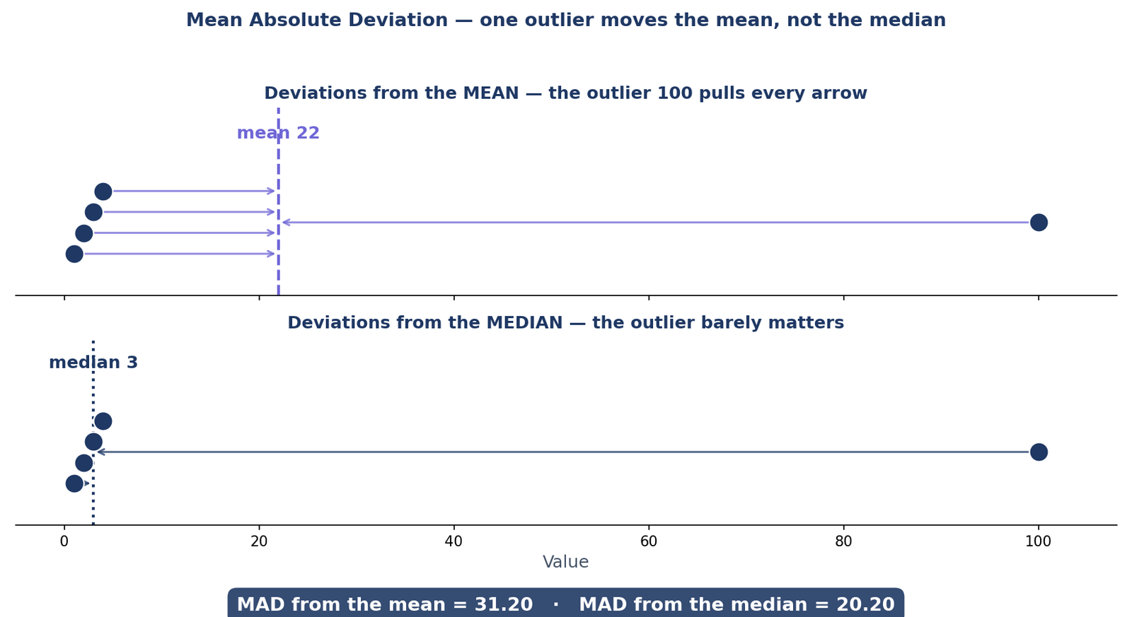
The picture below shows why that matters. Four of the five dots sit close together, but the single value of 100 drags the mean out to 22 while the median stays at 3 — and the two versions of MAD tell very different stories about the same data.
What Is Mean Absolute Deviation?
Mean absolute deviation — MAD for short — is the average distance between each value in a dataset and the dataset’s mean. Take every value, measure how far it sits from the mean, drop the sign so that distances below the mean count exactly the same as distances above it, and average those distances. The result is a single number, in the original units, that answers the question “how spread out is this data, typically?”
MAD = Σ|x − mean| ÷ n — add up the absolute deviation of every value from the mean, then divide by the number of values.
The absolute value is doing the essential work. Deviations from the mean always add up to exactly zero — values above the mean cancel values below it — so averaging the signed deviations would always give you nothing. Taking the absolute value first stops the cancellation and leaves a real measure of spread. On 2, 4, 6, 8, 10, the mean is 6 and the deviations are −4, −2, 0, +2 and +4; their absolute values are 4, 2, 0, 2 and 4, which average to 2.4. That is the whole trick, and it is why MAD is the easiest spread measure to explain to anyone: a MAD of 2.4 on test scores means a typical score sits 2.4 points from the mean. No squared units, no square roots, nothing to translate. If you want to check your own numbers, the mean absolute deviation calculator runs the same arithmetic and shows every deviation.
MAD is a measure of spread, so it belongs with the other summary numbers — mean, median and standard deviation — that a statistics calculator reports for a dataset. The difference is what MAD does with distance: it measures it directly, while standard deviation squares it first. That one choice changes everything about how the two measures behave, and the rest of this guide is about when each choice is the right one.
How to Calculate Mean Absolute Deviation Step by Step
Calculating MAD takes four steps and nothing more advanced than subtraction. Work through them once by hand and the formula stops being a symbol to memorize and becomes a procedure you understand.
- Find the mean. Add all the values together and divide by how many values there are.
- Find each absolute deviation. Subtract the mean from each value and drop the minus sign, so every deviation is a positive distance.
- Add the absolute deviations. Total all the distances from step 2.
- Divide by the number of values. That average is the mean absolute deviation.
Worked example: find the MAD of 2, 4, 6, 8, 10. The mean is (2 + 4 + 6 + 8 + 10) ÷ 5 = 6.
| Value | Deviation from the mean (6) | Absolute deviation |
|---|---|---|
| 2 | −4 | 4 |
| 4 | −2 | 2 |
| 6 | 0 | 0 |
| 8 | +2 | 2 |
| 10 | +4 | 4 |
| Total | — | 12 |
The absolute deviations add to 12. Divide by the 5 values: 12 ÷ 5 = 2.4. So the MAD is 2.4 — a typical value sits 2.4 away from the mean of 6. Try the same four steps on −2, 1, 5, 8: the mean is 3, the absolute deviations are 5, 2, 2 and 5, and 14 ÷ 4 = 3.5. The steps are identical if you center on the median instead of the mean — only step 1 changes — and the next section shows all three versions side by side on the same datasets.
The Three Kinds of MAD, Side by Side
“MAD” is really three different statistics sharing one name, and they only agree when the data is symmetric. The first centers on the mean, the second centers on the median, and the third takes the median of the deviations themselves. Put them side by side on the same datasets and the differences jump out:
| Dataset | MAD from the mean | MAD from the median | Median absolute deviation | Sample SD |
|---|---|---|---|---|
| 2, 4, 6, 8, 10 | 2.4 | 2.4 | 2 | 3.16 |
| 1, 2, 3, 4, 100 | 31.20 | 20.20 | 1 | 43.62 |
| 10, 20, 30 | 6.67 | 6.67 | 10 | 10 |
| 1, 2, 2, 3, 3, 3, 4, 5, 9 | 1.63 | 1.44 | 1 | 2.35 |
On the symmetric sets (2, 4, 6, 8, 10 and 10, 20, 30) the two MADs are identical, because the mean and the median are the same number. On the skewed sets they split apart — and the median absolute deviation splits furthest of all. On 1, 2, 3, 4, 100, the mean-based MAD says 31.20, the median-based MAD says 20.20, and the median absolute deviation says just 1. All three are honest answers to slightly different questions: the first asks how far values sit from the mean, the second how far they sit from the median, and the third how far a typical value sits from the median.
What Is Median Absolute Deviation?
Median absolute deviation is the median of the absolute deviations from the median. Take the dataset 1, 2, 3, 4, 100: its median is 3, so the absolute deviations are 2, 1, 0, 1 and 97. Sort them — 0, 1, 1, 2, 97 — and take the middle one: 1. A typical value is just 1 away from the median, and the lone value of 100 barely registers, because the median of the deviations only cares about the middle deviation, not the biggest one. That makes it the most outlier-proof spread measure in common use, and the one the NIST Engineering Statistics Handbook lists among the robust measures of scale, alongside the interquartile range.
Watch out for the name collision: many sources use “MAD” for both the mean version and this median version, and some use it for the median absolute deviation too. Always check which center a source is using before you compare numbers — a “MAD of 31.2” and a “MAD of 1” can describe the very same dataset. Which center to use is the same question as mean vs median vs mode: the mean is the natural center for symmetric data, the median for skewed data. The mean absolute deviation calculator reports all three versions for any dataset you paste in, so you can see them disagree in real time. And if you need a standard-deviation estimate from the median version, there is a fixed conversion for normal data: σ ≈ 1.4826 × median absolute deviation, which the next section covers in full.
What Is the Difference Between MAD and Standard Deviation?
MAD and standard deviation both measure spread, and both start from the same place: the deviations of each value from the mean. They differ in exactly one choice — what they do with those deviations. MAD takes the absolute value and averages. Standard deviation squares them, averages, and takes the square root. That single choice explains every difference between them.
In a normal distribution, MAD = σ × √(2/π) ≈ 0.7979σ — about 80% of the standard deviation (Geary, 1935). Turned around: σ ≈ 1.2533 × MAD.
The constants give you a way to move between the two measures when the data is roughly normal. On 2, 4, 6, 8, 10, the MAD is 2.4, so 1.2533 × 2.4 = 3.008, and the median absolute deviation is 2, so 1.4826 × 2 = 2.965 — the true sample standard deviation is 3.1623, so both estimates land close. On the outlier set 1, 2, 3, 4, 100, the mean-based conversion still works: 1.2533 × 31.2 = 39.1 against the true sample SD of 43.62. But the median-based conversion gives 1.4826 × 1 = 1.48, which is nowhere near 43.62. That is the point, not a mistake: the median version is nearly blind to the outlier, so converting it into a σ pretends the outlier does not exist.
MAD also has a blind spot of its own: two datasets can have the same MAD and different standard deviations. Take 5, 5, 9, 9 and 4, 6, 8, 10. Both have mean 7, and both have MAD 2 — the first has deviations of 2, 2, 2, 2 and the second has 3, 1, 1, 3. But their population standard deviations are 2.00 and 2.24: squaring punishes the 3s more than the 1s, so the dataset with the more extreme values gets the bigger SD. MAD only sees the average distance; it cannot see the shape of the spread.
| Mean absolute deviation | Standard deviation | |
|---|---|---|
| What it averages | Absolute deviations | Squared deviations (then square-rooted) |
| Units | Original units | Original units (variance is squared units) |
| Outliers | One value moves it in proportion | One value can dominate it |
| Role in normal theory | None directly | Defines the 68-95-99.7 bands and z-scores |
| Optimization | Kink at zero — hard to optimize | Smooth — easy to optimize |
The two measures are not rivals; they are tools for different jobs. The NIST Engineering Statistics Handbook lists median absolute deviation, average absolute deviation and the interquartile range as robust measures of scale — the right choice when the data may contain surprises. Standard deviation is the right choice when you need the machinery built on it: the empirical rule and Chebyshev’s theorem are both written in standard deviations, and so is every z-score.
Mean Absolute Deviation With Outliers
One outlier is the fastest way to see what MAD does — and what it cannot do. Take 1, 2, 3, 4, 100, the dataset in the diagram at the top of this guide. Its mean is 22, and the deviations from that mean are:
| Value | Deviation from the mean (22) | Absolute deviation |
|---|---|---|
| 1 | −21 | 21 |
| 2 | −20 | 20 |
| 3 | −19 | 19 |
| 4 | −18 | 18 |
| 100 | +78 | 78 |
| Total | — | 156 |
156 ÷ 5 = 31.20. The outlier moves MAD(mean) from 1.00 (without 100) to 31.20 — a thirty-fold jump from a single value. Without the 100, the four remaining values have mean 2.5 and deviations of 1.5, 0.5, 0.5 and 1.5, which average to exactly 1.00. So MAD is more forgiving than standard deviation, not immune to outliers: the sample standard deviation jumps from 1.29 to 43.62 on the same change. What MAD does is keep the damage proportional — the outlier contributes its distance, 78, and nothing more. Squaring it, as standard deviation does, would contribute 78² = 6,084.
Center on the median instead and the damage shrinks: the median is 3, the absolute deviations are 2, 1, 0, 1 and 97, and they average to 101 ÷ 5 = 20.20. Go one step further to the median absolute deviation and the outlier disappears entirely — it is 1 with the 100 in the data and 1 without it. The diagram at the top of this guide shows exactly this: the mean is dragged out to 22 while the median stays at 3.
Not every large value is a disaster. In 1, 2, 2, 3, 3, 3, 4, 5, 9, the 9 is the largest value but only a mild outlier, and MAD(mean) is 1.63 while MAD(median) is 1.44 — close together, and both sensible. The same dataset is worked in full, with every summary output and not just MAD, in What Is a Statistics Calculator? A single extreme value also drives the skewness of a dataset; you can measure that skew with the skewness and kurtosis calculator.
How to Calculate MAD for Grouped Data
When data arrives as a frequency table — test scores grouped by mark, ages grouped by year — you cannot list every value, but you can still find the MAD. Weight each absolute deviation by how often its value occurs:
Grouped MAD = Σ(f × |x − mean|) ÷ Σf — multiply each absolute deviation by its frequency, add them up, and divide by the total frequency.
Worked example: the values 10, 20, 30 and 40 occur 2, 3, 4 and 1 times. The mean is (10×2 + 20×3 + 30×4 + 40×1) ÷ 10 = 240 ÷ 10 = 24.
| Value (x) | Frequency (f) | |x − 24| | f × |x − 24| |
|---|---|---|---|
| 10 | 2 | 14 | 28 |
| 20 | 3 | 4 | 12 |
| 30 | 4 | 6 | 24 |
| 40 | 1 | 16 | 16 |
| Total | 10 | — | 80 |
The weighted deviations add to 28 + 12 + 24 + 16 = 80, and the total frequency is 10, so the grouped MAD is 80 ÷ 10 = 8. If the data is grouped into class intervals instead of single values, use the midpoint of each interval as x; the arithmetic is exactly the same.
Mean Absolute Deviation in Excel
Excel has a built-in function for MAD from the mean: =AVEDEV(range) returns the average of the absolute deviations of the data points from their mean. Put 2, 4, 6, 8, 10 in cells A1:A5 and =AVEDEV(A1:A5) returns 2.4 — exactly the value worked out by hand above. Note that AVEDEV always centers on the mean and divides by n, the number of values; there is no sample-versus-population choice the way there is for standard deviation.
There is no built-in Excel function for the other two versions, but both are one array formula away. For the median absolute deviation, use =MEDIAN(ABS(A1:A5-MEDIAN(A1:A5))): the inner part builds the list of absolute deviations from the median, and MEDIAN takes the middle one. For MAD from the median, use =AVERAGE(ABS(A1:A5-MEDIAN(A1:A5))): the same list of deviations, averaged instead. In modern Excel both work as ordinary formulas; in older versions, confirm them with Ctrl+Shift+Enter.
The same arithmetic shows up in forecasting and machine learning as mean absolute error (MAE): the average of |actual − predicted| instead of |value − mean|. MAD is MAE with the mean as the prediction, and both are judged in original units and forgiving of big misses compared with squared-error measures. That forgiveness is also why regression is usually fitted by least squares instead — the squared measure is smooth and easy to optimize, while the absolute value has a kink at zero. See linear regression explained for how least squares works.
When Should You Use MAD Instead of Standard Deviation?
Use MAD when the data may contain outliers or recording errors, when your audience needs a number in plain language (“a typical value is 2.4 away from the mean”), or when you are describing spread and nothing more. Use standard deviation when you need the machinery built on it — the empirical rule, z-scores, confidence intervals and hypothesis tests — when you are comparing the spread of roughly normal datasets, or when you are fitting a model. And when you need to compare spread across datasets with very different means, neither is ideal on its own: a relative measure such as the coefficient of variation is the right tool, and the coefficient of variation calculator computes it.
A practical rule of thumb: report both when they disagree. A large standard deviation next to a small MAD is itself information — it tells you the spread is driven by a few extreme values rather than by the bulk of the data, and that the median-based versions of MAD are probably the honest summary. When the two agree, either will do, and MAD is the easier one to explain.
Frequently Asked Questions
What is mean absolute deviation in simple terms?
It is the average distance between each value in a dataset and the mean. A MAD of 2.4 means a typical value sits 2.4 units from the mean — in the original units, with no squaring involved.
How do you calculate MAD step by step?
Find the mean, find each value’s absolute deviation from the mean, add those deviations, and divide by the number of values. On 2, 4, 6, 8, 10: the mean is 6, the absolute deviations are 4, 2, 0, 2 and 4, and 12 ÷ 5 = 2.4.
What is the MAD formula?
For raw data, MAD = Σ|x − mean| ÷ n. For grouped data, MAD = Σ(f × |x − mean|) ÷ Σf, weighting each absolute deviation by its frequency.
What is the difference between MAD from the mean and MAD from the median?
MAD from the mean centers on the mean; MAD from the median centers on the median. They are identical on symmetric data and split apart on skewed data — on 1, 2, 3, 4, 100 they are 31.20 and 20.20. The median version is the more robust of the two.
What is median absolute deviation, and how is it different?
It is the median of the absolute deviations from the median, not their average. On 1, 2, 3, 4, 100 it is 1, because the middle deviation is 1. It is the most outlier-proof of the three MADs, and for normal data σ ≈ 1.4826 × median absolute deviation.
How is MAD related to standard deviation?
In a normal distribution MAD is about 80% of the standard deviation (MAD ≈ 0.7979σ, Geary 1935), so σ ≈ 1.2533 × MAD. The two measure the same idea — spread — but MAD averages absolute distances while standard deviation averages squared distances.
Why use MAD instead of SD?
Because it stays in the original units, it is easy to explain, and one outlier moves it in proportion instead of dominating it. But standard deviation wins whenever you need normal-distribution theory: the empirical rule, z-scores, confidence intervals and hypothesis tests are all written in standard deviations.
How do you calculate MAD in Excel?
Use =AVEDEV(range) for MAD from the mean — =AVEDEV(A1:A5) returns 2.4 for 2, 4, 6, 8, 10. There is no built-in function for the median versions; use =MEDIAN(ABS(range-MEDIAN(range))) for the median absolute deviation and =AVERAGE(ABS(range-MEDIAN(range))) for MAD from the median.
Check Tools
Try the calculators behind this guide:
Mean Absolute Deviation Calculator
All three MADs, every deviation and the σ estimates for any dataset.
Try the Mean Absolute Deviation Calculator →
Statistics Calculator
The full summary — mean, median, mode, SD, CV and more — in one step.
Try the Statistics Calculator →
Coefficient of Variation Calculator
Compare relative spread across datasets with different means.
Try the Coefficient of Variation Calculator →
Skewness and Kurtosis Calculator
Measure the skew that a single outlier creates.
Try the Skewness and Kurtosis Calculator →
Check Articles
Keep reading with these guides from the site:
What Is a Statistics Calculator?
How to read every output — mean, median, mode, SD, CV — with a fully worked example.
Read What Is a Statistics Calculator? →
Mean vs Median vs Mode
Which center to quote, and when each one wins.
Read Mean vs Median vs Mode →
What Is Coefficient of Variation?
Relative spread, explained with worked examples.
Read What Is Coefficient of Variation? →
Chebyshev’s Theorem Explained
What spread guarantees when the data is not normal.
Read Chebyshev’s Theorem Explained →
Linear Regression Explained
Least squares, MAE and what the fit really minimizes.
Read Linear Regression Explained →
What Is the Empirical Rule?
The 68-95-99.7 rule in full, with the exact percentages.
Read What Is the Empirical Rule? →