
What Is a Statistics Calculator?
What is a statistics calculator? It is the fastest way to summarize a dataset: paste in your numbers and it returns the mean, median, mode, standard deviation and more, with every step shown. This guide works through one dataset by hand so you know what each number means — and which one to quote.
A statistics calculator turns numbers into a summary — mean, median, mode, range, variance, standard deviation and more. For 1, 2, 2, 3, 3, 3, 4, 5, 9 it reports a mean of 3.56, a sample standard deviation of 2.35 and a CV of 66.13%. The skill is not running it; it is knowing which number to quote.
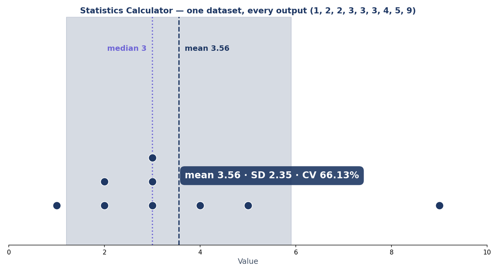
The picture below is the dataset this guide works through: nine values, most of them small, one of them — 9 — standing apart. The mean is 3.56, the median is 3, and the shaded band is one sample standard deviation either side of the mean, from 1.21 to 5.91.
What Is a Statistics Calculator?
A statistics calculator takes a list of numbers and returns a complete descriptive summary in one step: how many values there are, their sum, where their center sits, how spread out they are, and what shape the distribution has. You paste in the data — test scores, measurements, survey responses — and the statistics calculator does the arithmetic and shows every step, so you can check its work instead of trusting a black box.
The outputs fall into three groups. Center: the mean, the median and the mode — three different answers to “what is a typical value?” Spread: the range, the quartiles and the interquartile range, the variance and standard deviation, the standard error, the coefficient of variation and the mean absolute deviation — different answers to “how far apart are the values?” Shape: skewness and kurtosis — “is the distribution lopsided, and how heavy are its tails?” The next section works through all three groups on one dataset, number by number.
One boundary matters: a statistics calculator is descriptive. It summarizes the data you have; it does not test hypotheses, estimate population parameters or tell you whether a difference is real. For that you need inferential tools — a p-value calculator, and the guide to what a p-value is before you use one.
The Complete Worked Summary: One Dataset, Every Output
Here is the whole summary for 1, 2, 2, 3, 3, 3, 4, 5, 9 — the same numbers the statistics calculator reports, worked by hand so you can see where each one comes from. The values are already sorted, n = 9 and the sum is 32.
| Output | Value |
|---|---|
| Count (n) | 9 |
| Sum | 32 |
| Mean | 3.56 |
| Median | 3 |
| Mode | 3 |
| Range | 8 |
| First quartile (Q1) | 2 |
| Third quartile (Q3) | 4 |
| Interquartile range (IQR) | 2 |
| Sum of squared deviations (SS) | 44.222 |
| Population variance | 4.914 |
| Sample variance | 5.528 |
| Population SD | 2.22 |
| Sample SD | 2.35 |
| Standard error | 0.78 |
| Coefficient of variation | 66.13% |
| Skewness (Fisher) | 1.728 |
| Excess kurtosis | 3.648 |
| MAD (from the mean) | 1.63 |
| MAD (from the median) | 1.44 |
How the numbers are built. Add the values (32) and divide by 9 for the mean, 3.5556 — reported as 3.56. The median is the 5th value, 3; the mode is 3, the only value that repeats three times; the range is 9 − 1 = 8. The quartiles use the median-of-halves method the calculator uses: split the sorted data at the median (3), counting the median itself in both halves — the lower half (1, 2, 2, 3, 3) has median 2 and the upper half (3, 3, 4, 5, 9) has median 4, so Q1 = 2, Q3 = 4 and IQR = 2. Tukey’s hinges, which exclude the median from both halves, give Q3 = 4.5 — different tools can report different quartiles for the same data, and that is normal. The squared deviations from the mean add to SS = 44.222; divide by 9 for the population variance (4.914) and by 8 for the sample variance (5.528), and the square roots give the two standard deviations, 2.22 and 2.35. The standard error is 2.351 ÷ √9 = 0.78, and the CV is 2.351 ÷ 3.556 × 100 = 66.13%. The two MADs — 1.63 from the mean and 1.44 from the median — are worked in full in Mean Absolute Deviation Explained, and the mean absolute deviation calculator computes them for any dataset. Keep this table in mind: every section that follows explains one row of it in depth.
How to Use a Statistics Calculator
Using the calculator takes four steps and no statistical background. The skill is not in the clicking — it is in reading the summary that comes back, which the next three sections teach.
- Paste your data. Type or paste the numbers into the input box, separated by commas, spaces or new lines — the calculator accepts them all.
- Choose population or sample. Tell the calculator whether your numbers are the whole group or a sample of a bigger one; it changes the variance and standard deviation. When in doubt, pick sample.
- Click Calculate. The calculator sorts the values, finds the center and spread, and draws the dot plot.
- Read the summary. Start with the mean and median, then the standard deviation and CV, then the shape numbers — the next three sections explain each one.
A second example shows the same outputs on symmetric data. For 2, 4, 6, 8, 10 — the calculator’s own worked example — the mean and median are both 6, the range is 8, the population standard deviation is 2.83 and the sample standard deviation is 3.16, the population variance is 8 and the sample variance is 10, the quartiles are Q1 = 4 and Q3 = 8 (so IQR = 4), the standard error is 1.41 and the CV is 52.70%. Skewness is 0 — the data is perfectly symmetric — and the excess kurtosis is −1.2. Compare that with the main example’s CV of 66.13% and skewness of 1.728: the symmetric set is tighter and balanced, while the skewed set is spread out and lopsided. Try both datasets in the statistics calculator and watch how the outputs move.
The same summary in Excel: =AVERAGE(range) for the mean, =MEDIAN(range) for the median, =MODE.SNGL(range) for the mode, =STDEV.P(range) for the population standard deviation, =STDEV.S(range) for the sample standard deviation, and =DEVSQ(range) for the sum of squared deviations — the SS of 44.222 in the table above — which is the hand-check for both variances. A calculator is faster for a one-off summary; Excel is better when the data keeps changing or runs to thousands of rows.
Which Number Should I Quote — Mean, Median or Mode?
The three center numbers agree on the worked example — mean 3.56, median 3, mode 3 — but they often disagree, and the choice changes the story. Each one answers a different question, so the right quote depends on what you want to say:
| Situation | Quote | Why |
|---|---|---|
| Symmetric data, no outliers | Mean | Uses every value; the standard for inference |
| Skewed data or outliers | Median | Not dragged by extremes |
| Categories, or the most common value | Mode | The only center that works for categories |
| Comparing typical values across groups | Median (or the mean, if symmetric) | Robust comparison |
The house-price lesson makes the point. Nine houses priced from $250,000 to $272,000 have a mean of $261,556 and a median of $261,000 — the two agree, and either describes the market. Add one $2.1 million house and the mean jumps to $445,400, a 70% rise, while the median moves only to $262,000. The median barely notices the mansion; the mean is pulled up by it. That is why house prices are always reported as medians, and why quoting the mean for skewed data is the most common statistics mistake there is. The same logic applies to the worked example: the single value of 9 pulls the mean (3.56) above the median (3), which is the first hint that the data is skewed — the skewness of 1.728 confirms it.
The full comparison — with more examples of when each center wins — is in mean vs median vs mode. And remember that a single value is not a summary at all: see what is a raw score for the difference between one measurement and a summary of many.
Should I Use Population or Sample Standard Deviation?
The worked example reports two standard deviations — population 2.22 and sample 2.35 — and they come from the same sum of squared deviations (SS = 44.222). The difference is only the divisor: the population version divides by n, the number of values, while the sample version divides by n − 1.
Population variance = SS ÷ n; sample variance = SS ÷ (n − 1). The sample version is always a little bigger.
Use the population standard deviation when your numbers ARE the whole group — every student in the class, every item in the batch. Use the sample standard deviation when your numbers are a sample from something bigger — 20 voters surveyed out of thousands, 9 measurements standing in for a process. The sample version corrects a small-sample bias: values cluster a little tighter around the sample mean than around the true mean, so dividing by n would understate the spread, and n − 1 (Bessel’s correction) fixes it. When in doubt, pick sample — it is the safer default, and the calculator’s default. For large n the difference vanishes: at n = 100 the two differ by about 0.5%.
There is a case where neither standard deviation helps — and the mean fails too. The NIST Engineering Statistics Handbook shows a Cauchy sample whose mean is 3.70 but whose median is −0.016. The Cauchy distribution has such heavy tails that its mean is meaningless: a single extreme value can drag it anywhere, and more data does not settle it down. The median, at −0.016, is the honest center. When the mean and median disagree this wildly, quote the median and say so — the mean is not describing the data. The shape numbers that warn you about heavy tails are skewness and kurtosis, which you can measure with the skewness and kurtosis calculator.
What Does a High CV Tell You?
The coefficient of variation turns spread into a percentage of the mean — CV = sample SD ÷ mean × 100 — so you can compare datasets measured in different units. The worked set’s CV is 66.13%, which is high: as a rule of thumb, below about 10% is low, 10–30% is moderate, and above about 30% is high. A CV of 66.13% says the values are widely scattered relative to their average, and here the single value of 9 is doing most of that scattering. The symmetric set’s CV is 52.70% — also high, because its mean (6) is small next to its spread. The full guide is what is coefficient of variation, and the coefficient of variation calculator computes it for any dataset.
One caveat: the CV is meaningless when the mean is near zero — dividing by almost nothing makes the percentage explode — and misleading for data with negative values. In those cases, use the plain standard deviation instead.
What Standard Error, Skewness and Kurtosis Add
The standard error, 0.78 on the worked set, is the sample standard deviation divided by the square root of n — it measures how precisely the mean is estimated, not how spread out the data is. It shrinks as the sample grows: quadruple the sample to halve it. Skewness of 1.728 means the data is strongly right-skewed — the 9 pulls the tail to the right — and an excess kurtosis of 3.648 means heavy tails and a sharp peak. For the symmetric set the skewness is 0 and the excess kurtosis is −1.2, flat and light-tailed. Read together, the three shape numbers tell you whether the mean is a safe summary or not.
From Summary to Next Step: What to Do With These Numbers
A summary is a starting point, not a conclusion. Mean and standard deviation in hand, check the empirical rule: if the data is roughly normal, about 68% of values fall within one standard deviation of the mean. Skewness above 1, or a mean far from the median, means the data is not normal — consider a transform, or quote the median instead, and check what still holds with Chebyshev’s theorem, which works for any shape. A high CV means you should compare datasets carefully and prefer relative measures. And a summary that looks odd is a reason to plot the data before you believe it.
Mistakes to avoid: quoting the mean for skewed data; mixing up population and sample standard deviation (the calculator labels both — read the label); reading too much into a tiny sample — with n = 1 there is no spread to measure at all, and with n = 3 the standard deviation is mostly noise; and trusting a summary without looking at the data — the Cauchy sample above has a mean of 3.70 and a median of −0.016, and no single number tells you that story.
Frequently Asked Questions
What does a statistics calculator do?
It takes a list of numbers and returns a complete descriptive summary in one step: the count, the sum, the mean, the median, the mode, the range, the quartiles, the variance, the standard deviation, the standard error, the coefficient of variation, and the shape numbers — skewness, kurtosis and mean absolute deviation. The calculator on this site shows every step, so you can check its work.
What is the difference between population and sample standard deviation?
The population standard deviation divides the sum of squared deviations by n; the sample standard deviation divides by n − 1. Use the population version when your numbers ARE the whole group, and the sample version when they are a sample of something bigger. When in doubt, pick sample — it is the safer default. On the worked set the two are 2.22 and 2.35.
When should I report the median instead of the mean?
When the data is skewed or has outliers. The mean is dragged by extremes: nine houses priced from $250,000 to $272,000 have a mean of $261,556 and a median of $261,000; add one $2.1 million house and the mean jumps 70% to $445,400 while the median barely moves, to $262,000. When the mean and the median disagree that much, quote the median.
What is CV and when does it matter?
The coefficient of variation is the standard deviation divided by the mean, times 100. It matters when you want to compare the spread of datasets measured in different units — a CV of 66.13% on the worked set is high relative spread. It is meaningless when the mean is near zero or the data has negative values.
Can a dataset have more than one mode?
Yes. A dataset with two values tied for the most frequent is bimodal; three or more ties make it multimodal. A dataset with no repeats has no mode at all — the symmetric set 2, 4, 6, 8, 10 has no mode. The calculator reports the mode only when one exists.
What is standard error, and why does the calculator show it?
The standard error is the sample standard deviation divided by the square root of n. It measures how precisely the mean is estimated: 0.78 on the worked set. It is not a measure of spread — it shrinks as the sample grows, and you need it whenever you want to know how much the mean might move if you collected the data again.
Can a statistics calculator do hypothesis tests?
Not this one. The statistics calculator is descriptive: it summarizes the data you have and does no inference. For a test, use the p-value calculator — and read what is a p-value before you interpret the result.
Is a statistics calculator better than Excel?
For a one-off summary, yes: paste the numbers and every output appears at once, with the steps shown. For large or repeated data, Excel is better — =AVERAGE for the mean, =MEDIAN for the median, =MODE.SNGL for the mode, =STDEV.P and =STDEV.S for the two standard deviations, and =DEVSQ for the sum of squared deviations.
Check Tools
Run the summary on your own numbers:
Statistics Calculator
Run the full summary on your own numbers, with every step shown.
Open the Statistics Calculator →
Mean Absolute Deviation Calculator
The three MADs and the σ estimates for any dataset.
Open the Mean Absolute Deviation Calculator →
Coefficient of Variation Calculator
Compare spread across datasets measured in different units.
Open the Coefficient of Variation Calculator →
Skewness and Kurtosis Calculator
Measure the shape of your data — skew and tails.
Open the Skewness and Kurtosis Calculator →
Check Articles
Keep reading with these guides from the site:
Mean Absolute Deviation Explained
The formula, three kinds of MAD, and when MAD beats standard deviation.
Read Mean Absolute Deviation Explained →
Mean vs Median vs Mode
When each center wins, with more examples.
Read Mean vs Median vs Mode →
What Is Coefficient of Variation?
The full guide to CV and relative spread.
Read What Is Coefficient of Variation? →
What Is a Raw Score?
One measurement is not a summary — see the difference.
Read What Is a Raw Score? →
Chebyshev’s Theorem Explained
The rule that works for any distribution shape.
Read Chebyshev’s Theorem Explained →
What Is a P-Value?
What to do when your summary leads to a test.
Read What Is a P-Value? →