Confidence Interval for the Difference of Two Means
Welch is the safer default: it does not assume the two variances are equal.
Results
95%
-
-
-
-
-
-
-
-
Distribution of the difference
The shaded region is the confidence interval. The red dashed line marks a difference of 0.
Interpretation
Enter values and click calculate to see the interpretation.
Formula Used
CI = (x̄₁ − x̄₂) ± t* × SE
Welch (unequal variances): SE = √(s₁²/n₁ + s₂²/n₂), df by the Welch–Satterthwaite formula.
Pooled (equal variances): sp = √[((n₁−1)s₁² + (n₂−1)s₂²)/(n₁+n₂−2)], SE = sp × √(1/n₁ + 1/n₂), df = n₁ + n₂ − 2.
Verdict: if the interval contains 0, the difference is not statistically significant.
A confidence interval for the difference of two means estimates where the difference between two means (μ₁ − μ₂) lies. Enter mean, standard deviation and size, choose Welch or pooled, and pick a confidence level. Means of 75 and 70, with 30 observations each, give a 95% Welch interval of [−0.71, 10.71], which contains 0, so it is not significant.
The confidence interval for difference of two means calculator on this page builds a proper statistical interval from two samples. It offers both Welch (unequal variances) and pooled (equal variances) methods, and always uses the t-distribution, so the critical value t* adapts to each sample size: small samples get wider, more honest intervals, while large samples converge on the familiar z-values. Enter both sample means (x̄₁, x̄₂), standard deviations (s₁, s₂) and sample sizes (n₁, n₂) to get the difference, standard error, margin of error and both bounds instantly. If you only have a population mean and standard deviation and no sample size, use our empirical rule confidence interval calculator instead — that tool describes where data falls, while this one estimates where the true difference lies.
What Is a Confidence Interval for the Difference of Two Means?
A confidence interval (CI) for the difference of two means is a range of values, calculated from two samples, that is likely to contain the true difference between two population means (μ₁ − μ₂) with a stated level of confidence — usually 95%. It measures sampling uncertainty for the difference, and is always written as (x̄₁ − x̄₂) ± margin of error. A 95% interval of [−0.71, 10.71] does not mean that 95% of the data falls between −0.71 and 10.71. That job belongs to the empirical rule (68–95–99.7), which describes where data falls. A confidence interval is about the unknown difference, not the data: if you repeated both samples many times, about 95% of the intervals you built would contain the true difference. One single interval either contains the true difference or it does not — the 95% describes the long-run reliability of the method.
This is inferential statistics, not descriptive: you are estimating a population parameter — the difference μ₁ − μ₂ — from two samples. The wider the interval, the less precise the estimate. Because the calculator compares two samples, it must also allow for the fact that their variances may differ: the Welch method does this without assuming equal variances, while the pooled method assumes the two population variances are equal. If you only have one sample, use our confidence interval from mean and standard deviation calculator instead — it estimates a single population mean. To see the difference between describing data and estimating a parameter, read how the empirical rule differs from a confidence interval.
The most useful question the interval answers is whether the difference is real: if the interval contains 0, the two population means could plausibly be equal, and the difference is not statistically significant. The calculator gives this verdict with every result, so you do not need a separate two-sample t test to read it.
Formula for a Confidence Interval for the Difference of Two Means
The calculator uses one pattern for every confidence interval from sample statistics: centre the interval on the observed difference, then add and subtract a margin of error. This tool always uses the t-distribution version of the formula, because the standard deviations you enter are sample estimates (s₁, s₂), not known population values (σ₁, σ₂):
Welch formula — unequal variances (the default)
CI = (x̄₁ − x̄₂) ± t* × √(s₁²/n₁ + s₂²/n₂)
The critical value t* comes from the t-distribution with degrees of freedom from the Welch–Satterthwaite formula, so it adapts to both sample sizes and both spreads. Welch is the default because it stays valid even when the two variances are very different, and it loses almost no precision when they are equal.
Pooled formula — equal variances
CI = (x̄₁ − x̄₂) ± t* × sp × √(1/n₁ + 1/n₂), where sp = √[((n₁−1)s₁² + (n₂−1)s₂²)/(n₁+n₂−2)]
The pooled method first combines the two sample variances into one pooled standard deviation sp, then uses df = n₁ + n₂ − 2. Use it only when the two population variances are plausibly equal — for example, when the two samples come from the same measurement process. If the sample standard deviations differ by a lot, prefer Welch.
The t-interval above is the standard method for comparing two means when the standard deviations are estimated from the samples; it is the two-sample version of Student’s t interval, documented in the NIST/SEMATECH e-Handbook of Statistical Methods.
Terms
| Term | Meaning |
|---|---|
| x̄₁ | Sample mean of group 1 |
| s₁ | Sample standard deviation of group 1 (your estimate of σ₁) |
| n₁ | Sample size of group 1 |
| x̄₂ | Sample mean of group 2 |
| s₂ | Sample standard deviation of group 2 (your estimate of σ₂) |
| n₂ | Sample size of group 2 |
| sp | Pooled standard deviation (pooled method only) |
| df | Degrees of freedom: Welch–Satterthwaite (Welch) or n₁ + n₂ − 2 (pooled) |
| t* | Critical value from the t-distribution (depends on df and confidence level) |
| SE | Standard error of the difference: √(s₁²/n₁ + s₂²/n₂) (Welch) or sp × √(1/n₁ + 1/n₂) (pooled) |
| ME | Margin of error = t* × SE |
Critical values t* used by this calculator
| Degrees of freedom | 90% | 95% | 99% |
|---|---|---|---|
| 10 | 1.812 | 2.228 | 3.169 |
| 15 | 1.753 | 2.131 | 2.947 |
| 20 | 1.725 | 2.086 | 2.845 |
| 24 | 1.711 | 2.064 | 2.797 |
| 30 | 1.697 | 2.042 | 2.750 |
| 40 | 1.684 | 2.021 | 2.704 |
| 50 | 1.671 | 2.000 | 2.660 |
| 60 | 1.658 | 1.980 | 2.617 |
| Over 60 | 1.645 | 1.960 | 2.576 |
Read the row for your degrees of freedom. In Welch mode the df is usually not a whole number — the calculator uses the exact value, and rounds it for display: the worked example above has df = 56.2, so it reads between the 50 and 60 rows. In pooled mode df = n₁ + n₂ − 2 is always a whole number.
Rule of thumb: use Welch by default, and the pooled interval only when the two sample standard deviations are similar and the samples come from similar populations. Welch costs almost nothing when the variances are equal, but pooled can mislead when they are not. Use the t-formula whenever the standard deviation is estimated from your sample, which is almost always.
How to Use This Calculator
Follow these steps to calculate a confidence interval for the difference of two means:
- Enter the first sample’s mean (x̄₁) and standard deviation (s₁) — for example, 75 and 10.
- Enter the first sample size (n₁) — for example, 30.
- Enter the second sample’s mean (x̄₂), standard deviation (s₂) and size (n₂) — for example, 70, 12 and 30.
- Choose Welch or pooled — keep Welch unless the two variances are plausibly equal.
- Choose your confidence level — 90%, 95% or 99%, or pick Custom and type any level, such as 97.5%.
- Click “Calculate Confidence Interval”.
- Read the results — the difference, the standard error, the critical value t*, the degrees of freedom, the margin of error, the lower and upper bounds, the shaded curve, and the contains-0 verdict.
Note: the calculator always uses the t-distribution, because your standard deviations are estimated from the samples. If you know the population standard deviations instead, the z-formula applies — use our z-score calculator to turn a difference into a standard score.
Worked Examples: Three Intervals, Two Verdicts
Example 1 — the tool’s own numbers (Welch, 95%). Two samples: group 1 has a mean of 75, a standard deviation of 10 and n = 30; group 2 has a mean of 70, a standard deviation of 12 and n = 30. The difference is 75 − 70 = 5. The standard error is SE = √(10²/30 + 12²/30) = 2.85, the Welch degrees of freedom are df = 56.2, so t* = 2.00 and the margin of error is ME = 2.00 × 2.85 = 5.71. The interval is 5 ± 5.71 = [−0.71, 10.71]. We are 95% confident the true difference between the two population means lies between −0.71 and 10.71. Because the interval contains 0, the difference is not statistically significant.
Example 2 — a clear difference (Welch, 95%). Group 1: mean 100, standard deviation 15, n = 25; group 2: mean 90, standard deviation 15, n = 25. The difference is 10, the standard error is SE = √(15²/25 + 15²/25) = 4.24, df = 48 and t* = 2.01. The margin of error is 8.53, so the interval is 10 ± 8.53 = [1.47, 18.53]. This interval does not contain 0, so the difference is statistically significant — the first group’s population mean is plausibly 1.47 to 18.53 higher.
Example 3 — the same data, pooled (95%). Using Example 1’s numbers with the pooled method: the pooled standard deviation is sp = 11.05, the standard error is again 2.85, df = 30 + 30 − 2 = 58 and t* = 2.00, giving the same interval [−0.71, 10.71] to two decimal places. The two methods often agree when the samples are similar in size and spread — they diverge when the standard deviations or sample sizes differ a lot. Try it above: switch the method to pooled and watch the degrees of freedom change from 56 to 58.
Real-life example — an A/B test. A website tests two checkout designs. Design A has a mean order value of £84.60 (s = £12.40, n = 120) and design B £78.30 (s = £11.80, n = 120). The difference is £6.30, the Welch standard error is £1.56, df = 237 and t* = 1.97, giving a 95% interval of [£3.22, £9.38]. The interval does not contain 0, so design A is significantly better — and the interval shows the gain is at least about £3.22 per order.
What happens when the sample grows? With the same means and standard deviations as Example 1, doubling both samples to n = 60 each shrinks the standard error from 2.85 to about 2.02 and the margin of error from 5.71 to about 3.99, giving [1.01, 8.99] — now the interval excludes 0. Quadrupling a sample roughly halves the margin of error, because the standard error divides by √n.
How to read the results. The calculator returns the confidence level, the critical value t*, the standard error, the margin of error and both bounds. The interval itself is the two bounds: the lower bound is the difference minus the margin of error, and the upper bound is the difference plus the margin of error. The interpretation sentence underneath says it plainly — “We are 95% confident that the true difference between the two population means lies between…” — use that sentence in your report, and always quote the confidence level and the method (Welch or pooled) with it. The shaded curve shows the sampling distribution of the difference, with the interval shaded and a red dashed line at 0.
What makes the interval wider or narrower? Three things: the confidence level (99% is wider than 95% because t* is larger), the standard deviations (larger samples that vary more produce a larger standard error), and the sample sizes (larger samples make the interval narrower). If two samples have very different sizes, the smaller one dominates the standard error — the Welch standard error is √(s₁²/n₁ + s₂²/n₂), so a small n₁ with a large s₁ widens the interval more than a large n₂ can narrow it.
Common mistakes. Do not say “there is a 95% probability the true difference is in this interval” — the 95% describes the method, not this particular interval, which either contains the truth or does not. Do not use the pooled method just because it gives a neater degrees of freedom: if the two standard deviations differ by more than about a factor of two, Welch is the safer choice. Do not run a separate t test to decide significance when the interval already tells you — if it contains 0, the difference is not significant at that confidence level. And use the margin of error calculator if you want to plan a sample size around a target precision instead.
Empirical Rule vs Confidence Interval (Connection Section)
| Aspect | Empirical Rule | Confidence Interval |
|---|---|---|
| Purpose | Describes data spread in a population | Estimates the difference between two population means from two samples |
| Input | Population mean (μ), SD (σ) | Two sample means (x̄₁, x̄₂), SDs (s₁, s₂), sizes (n₁, n₂) |
| Output | % of data in range (68%, 95%, 99.7%) | Range likely containing the true difference μ₁ − μ₂ |
| Type | Descriptive | Inferential |
| Assumption | Normal distribution | Normal sampling distribution |
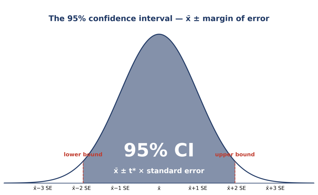
Key insight: the 68–95–99.7 rule tells you where data falls; a confidence interval tells you where the true difference between two means likely is. One describes the data you have; the other estimates the population value you do not have. The diagram at the top of this page shows the interval on the curve: the shaded middle 95% is the confidence interval, and the red dashed line marks a difference of 0.
Compare this exact interval with our population-style interval for estimated coverage, or read the full comparison in empirical rule vs confidence interval.
Common Confidence Levels
| Confidence Level | Z-Value | T-Value (df=20) | Use Case |
|---|---|---|---|
| 90% | 1.645 | ~1.725 | Moderate precision |
| 95% | 1.96 | ~2.086 | Standard in research |
| 99% | 2.576 | ~2.845 | High certainty |
The Z-Value column shows the large-sample limit. For the exact t* for your own sample size, use the critical-value table above — with df = 48 the 95% t* is 2.01, not 1.96. To use any other level, such as 97.5% or 80%, choose Custom in the calculator above and type the percentage. For a closer look at how the margin of error and the confidence level trade off, read margin of error vs confidence interval.
When to Use This Calculator
Use the confidence interval for difference of two means calculator when:
- Comparing two groups — treatment vs control, design A vs design B, before vs after.
- Reporting statistical precision in research papers, lab reports and business experiments.
- Estimating population differences in quality control, medicine and product analytics.
- Performing hypothesis testing with a margin of error — the contains-0 verdict is a two-sided test at your chosen level.
It is essential in statistical modelling, data science and scientific research. If you are comparing proportions instead of means, use the one-proportion z-test calculator to test a single proportion, and check the strength of the evidence with our p-value calculator from z-score. If you need a percentile for a single value instead, use the empirical rule percentile calculator or visualise percentiles on a normal distribution.
How do you calculate a confidence interval for the difference of two means?
Take the difference of the two sample means, then add and subtract t* × SE. With Welch, SE = √(s₁²/n₁ + s₂²/n₂) and the degrees of freedom come from the Welch–Satterthwaite formula; with pooled, the two variances are first combined into sp and df = n₁ + n₂ − 2. For example, means of 75 and 70 with standard deviations of 10 and 12 and 30 observations each give SE = 2.85, t* = 2.00 and a 95% interval of [−0.71, 10.71].
What does it mean if a confidence interval for the difference of two means contains 0?
It means 0 is a plausible value for the true difference — the two population means could be equal, so the difference is not statistically significant at that confidence level. It does not prove the means are equal; it only says the data do not rule out equality. A narrower interval that still contains 0 is stronger evidence of a small difference than a wide one.
Should I use Welch or pooled for a confidence interval for the difference of two means?
Use Welch by default. It does not assume the two population variances are equal, and it loses almost no precision when they are equal. Use pooled only when you have a clear reason to believe the variances are equal, for example when both samples come from the same measurement process and their standard deviations are similar. If the standard deviations differ by a lot, pooled intervals can be misleadingly narrow.
FAQs
Enter both samples’ means, standard deviations and sizes into the calculator above, choose Welch or pooled and a confidence level (90%, 95% or 99%, or Custom), then click Calculate Confidence Interval. The calculator works out the difference, the standard error, the t critical value for your degrees of freedom and the margin of error, then shows the lower and upper bounds, a shaded curve and a contains-0 verdict.
Welch uses SE = √(s₁²/n₁ + s₂²/n₂) with degrees of freedom from the Welch–Satterthwaite formula and does not assume equal variances. Pooled first combines the two sample variances into one pooled standard deviation sp, then uses SE = sp × √(1/n₁ + 1/n₂) with df = n₁ + n₂ − 2. Use Welch by default; use pooled only when the two population variances are plausibly equal.
95% is the standard choice in research and reporting. Use 90% when you want a narrower interval and can accept more uncertainty, and 99% when you need high certainty and can accept a wider interval. A higher confidence level always widens the interval.
No — this tool needs sample statistics (means, standard deviations and sizes from two samples). If you have the population mean and standard deviation and no sample size, use our empirical rule confidence interval calculator, which describes where data falls in a normal distribution.
The empirical rule describes where data in a normal population falls (about 68% within one standard deviation, 95% within two). A confidence interval estimates where the true difference between two population means lies, with a stated level of confidence. One is descriptive; the other is inferential.
A wide interval comes from small samples, large standard deviations or a high confidence level. The most effective fix is a larger sample size: quadrupling each sample roughly halves the margin of error, because the standard error divides by √n.
Roughly, each group needs n ≈ (t* × s / ME)² observations. With a standard deviation of about 11 and a 95% t* of about 2, that is (2 × 11 / 2)² ≈ 121 — about 120 observations per group. Use the margin of error calculator on this site to plan it precisely.
Yes — and that is often the most useful outcome. If the interval contains 0, the two population means could plausibly be equal and the difference is not statistically significant at that confidence level. If it excludes 0, the difference is statistically significant.
Related Tools
Explore these related calculators:
Confidence Interval from Mean and Standard Deviation Calculator: Estimate a confidence interval for a single population mean from a sample mean, standard deviation and size.
Margin of Error Calculator: Work out the margin of error for your next survey or experiment before you collect the data.
Empirical Rule Confidence Interval Calculator: Estimate 68%, 95% and 99.7% coverage from a population mean and standard deviation.
Empirical Rule vs Confidence Interval: Learn how the empirical rule differs from a confidence interval — and when to use each one.
Conclusion
The confidence interval for difference of two means calculator is a powerful tool for inferential statistics, enabling precise estimation of the difference between two population means from sample data. Whether you are in research, quality control or data science, you now know how to build a t-based interval with Welch or pooled variances, read its standard error and margin of error, and explain what the confidence level — and the contains-0 verdict — really means. For population-level descriptions, compare your results with the empirical rule view — and to keep exploring, browse all 33 free statistics tools.
Empirical Rule Calculator
Explore our statistical tools: calculate percentiles, visualize bell curves, and plot z-scores with simple, accurate calculators for normal distributions.
Try CalculatorEmpirical Rule Graph Generator
Visualize the 68-95-99.7 Rule with a bell curve showing standard deviation intervals. Great for quick insights and presentations.
Try CalculatorBell Curve Generator
Create customizable bell curve plots for any normal distribution. Perfect for data analysis and visual reports.
Standard Deviation Shading Tool
Shade areas under the curve based on standard deviation. Instantly see data coverage between values.
Try Calculator